I think blogging about my first time digging into reinforcement learning (RL) theory would be fun. So boom, here it goes!

This post begins with the classic Markov decision process (MDP) formulation, moves through dynamic programming and Monte Carlo Methods, and then uses those ideas to arrive at temporal-difference learning.

Markov Decision Processes

Problem Framing

The reinforcement learning (RL) problem is meant to be a straightforward framing of the problem of learning from interaction to achieve a goal, or more vividly, “trial and error”.

The learner and decision-maker is called the agent. The thing it interacts with, comprising everything outside the agent, is called the environment. These two interact at each of a sequence of discrete time steps, \(t=0,1,2,3,\dots\). At each time step \(t\), the agent receives some representation of the environment’s state, \(S_t\in\mathcal{S}\), where \(\mathcal{S}\) is the set of possible states, and on that basis selects an action, \(A_t\in\mathcal{A}(S_t)\), where \(\mathcal{A}(S_t)\) is the set of actions available in state \(S_t\). One time step later, in part as a consequence of its action, the agent receives a numerical reward, \(R_{t+1}\in\mathcal{R}\subset\mathbb{R}\), and finds itself in a new state, \(S_{t+1}\).

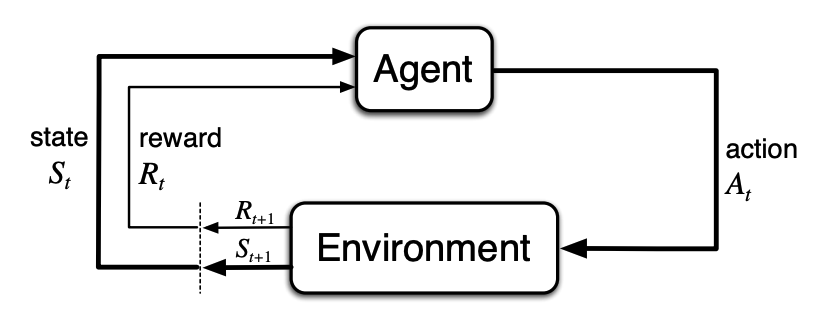
Consider the situation when the system starts at a particular state \(S_t\in\mathcal{S}\) and continuously taking actions after time step \(t\), resulting in a trajectory like

In general, we seek to maximize the expected return, where \(G_t\) can be defined in the simplest case as the cumulative reward the agent receives after time step \(t\):

where \(T\) is the final time step.

Since this expected return will be infinite when \(T=\infty\), the learning process above would possibly fail. In order to prevent this from happening, we introduce a parameter called the discount rate \(0\leq\gamma\leq 1\) to (1) as:

If \(\gamma<1\), the infinite sum has a finite value as long as the reward sequence \(\{R_k\}\) is bounded. If \(\gamma=0\), the agent is “myopic” in being concerned only with maximizing immediate rewards. As \(\gamma\) approaches \(1\), the objective takes future rewards into account more strongly: the agent becomes more farsighted.

The Markov Property

In the RL framework, the agent makes its decisions as a function of a signal from the environment’s state. In broad sense, “the state” means whatever information that is available to the agent. And we expect the state satisfies the Markov property, which we defined as follow.

Consider the response given by a general environment at time \({t+1}\) to the action taken at time \(t\), which may depend on everything that has happened earlier. In this case the dynamics can be defined as:

for all possible \(r\) and \(s^\prime\). If the environment’s response at \(t+1\) depends only on the state and action representations at \(t\), i.e.

for all \(s^\prime,r,S_t,A_t\), we say the state signal has the Markov property and is a Markov state.

A reinforcement learning task that satisfies the Markov property is called a Markov decision process (MDP), which models how a system changes state when different actions are applied. Formally, given any state \(s\) and action \(a\), the dynamics of an MDP can be specified by:

Value Functions

The value function of a state (or state-action pair) estimates how good or bad an individual is in a given state (or how good it is to perform a given action in a given state). And the notion of “how good” here is defined in terms of expected returns when starting in a specific state and following a specific behavior thereafter. Formally, we call this kind of behavior as a policy, \(\pi(a\vert s)\), which is a conditional distribution over the actions \(a\in\mathcal{A}\) given the state \(s\in\mathcal{S}\).

For MDPs, we can define the value of a state \(s\) under a policy \(\pi\) as

where \(\mathbb{E}_\pi\) denotes the expected value of a random variable given that the agent follows policy \(\pi\), and \(t\) is any time step. The function \(v_\pi\) is called the state-value function for policy \(\pi\).

Similarly, we define the value of taking action \(a\) in state \(s\) under a policy \(\pi\) as

The function \(q_\pi\) is called the action-value function for policy \(\pi\).

A fundamental property of value functions is that they satisfy particular recursive relationships. The value function can be mathematically decomposed into

which is the foundation of dynamic programming upon which all RL algorithms are based. This is the Bellman equation for \(v_\pi\), which expresses a relationship between the value of the state and the values of its successor state.

Optimal Policy

Solving a RL task roughly means finding an optimal policy \(\pi^*\) that maximize the expected return, which shares the same state-value function

and the same action value function

Intuitively, the value of a state under an optimal policy must equal the expected return for the best action from that state. Starting from this fact, we can derive the so-called Bellman optimality equation for \(v^*\):

Similarly, we can also derive the Bellman optimality equation for \(q^*\) is

The Bellman optimality equation is actually a system of equations with \(N\) equations and \(N\) unknowns. By solving this system of nonlinear equations, we can get \(v^*\) and \(q^*\), which determine an optimal policy.

Dynamic Programming

The key idea of RL generally, is the use of value functions to organize and structure the search for good policies. Dynamic programming (DP) refers to a collection of algorithms that can be used to compute the value functions defined earlier, given a perfect model of the environment as an MDP.

Policy Iteration

Policy iteration is one of the ways of finding an optimal policy, which mainly consists of two components, evaluation and improvement. Basically, we hope to achieve that through a sequence:

where \(\xrightarrow{E}\) denotes a policy evaluation and \(\xrightarrow{I}\) denotes a policy improvement.

Policy Evaluation

Consider how to compute the state-value function \(v_\pi\) for an arbitrary policy \(\pi\), which is commonly called policy evaluation. Recall that the Bellman equation for \(v_\pi\) is formed as

Since both the policy term \(\pi(a\vert s)\) and the environment’s dynamics term \(p(s^\prime,r\vert s, a)\) are completely known, this form is actually a system of \(\vert\mathcal{S}\vert\) linear equations in \(\vert\mathcal{S}\vert\) unknowns (\(v_\pi(s),s\in\mathcal{S}\)). If we arrange state values, rewards and transition probabilities ​​into matrices:

where

then the Bellman equation can be written into the matrix form:

Thus we find the solution as:

Then methods like Gaussian elimination are applied in the linear algebra literature. But RL typically deals with a vast state space (\(\vert\mathcal{S}\vert\) is very large) and does not necessarily require an exact solution.

Let’s take a deeper look inside. Define the Bellman expectation operator \(T_\pi\) as

where \(v:\mathcal{S}\to\mathbb{R}\) is a random value function. If we let \(v=v_\pi\), then we have

Obviously, \(v_\pi\) is exactly the fixed-point of \(T_\pi\). So for our purposes, methods like fixed-point iteration are most suitable, since the Bellman equation in matrix form is hoped to converge to the fixed-point \(\mathbf{v}_\pi\).

The detailed iteration algorithm is described as follow:

Policy Improvement

Intuitively, we hope the policy gets better and better through the “trial and error” process. Since we are able to compute \(v_\pi\) for a policy \(\pi\) through policy evaluation, we are able to tell a new policy \(\pi^\prime\) is better if

which is to say, starting from any state, the expected return of executing \(\pi^\prime\) is no less than that of executing \(\pi\). This means a complete iteration algorithm needs to be performed again. The value of the policy improvement theorem lies in the fact that we only need to know \(v_\pi\) or \(q_\pi\) of the old policy to determine whether a certain modification guarantees a better policy.

Policy improvement theorem. Let \(\pi\) and \(\pi^\prime\) be any pair of policies such that

then the policy \(\pi^\prime\) must be as good as, or better than, \(\pi\). The proof goes as follow:

Within this theorem, we can easily construct a greedy policy \(\pi^\prime\) by selecting at each state the action that appears the best:

which is also known as one-step lookahead. In particular, if the new greedy policy \(\pi^\prime\) is as good as the old policy \(\pi\), then we have

which is exactly the same as the Bellman optimality equation. This indicates that we’ve already find the optimal policy.

Value Iteration

In essence, policy evaluation is just repeatedly applying Bellman expectation operator to the estimated state-value until convergence, i.e.

where \(m\) tends towards infinity. This process introduces most of the cost during policy iteration. And in fact, it’s possible to truncate the evaluation process.

Policy improvement does not require high precision for every state-value. Consider two possible actions at a certain state. Even if the value estimation is still biased, as long as the judgment that one action is better than the other remains unchanged, continuing to calculate \(V\) more accurately will not change the next strategy improvement. Therefore, we can pre-set an \(m\), thus only performing a limited number of evaluations. And value iteration is a special case of policy iteration that \(m\) is set to be \(1\), cutting off policy evaluation to only one round.

We can write the detailed algorithm as follow:

Monte Carlo Methods

Monte Carlo methods are ways of solving the reinforcement learning problem based on averaging sample returns. Unlike DP, where we assume complete knowledge of the environment, Monte Carlo methods require only experience (sample sequences of states, actions, and rewards from actual or simulated interaction with an environment).

Monte Carlo Prediction

Let’s consider the policy evaluation problem again. First we define an episode as one complete journey or trial where an agent interacts with its environment, starting from an initial state and ending at a terminal state. And we call each occurrence of a certain state s in an episode a visit to s.

Assume we already have a set of \(n\) episodes obtained by following \(\pi\) and passing through \(s\). To estimate \(v_\pi(s)\), the value of a certain state \(s\) under a given policy \(\pi\), we can simply average the returns observed after visits to that state. As more returns are observed, the average should converge to the expected value. In particular, we introduce first-visit MC method, which estimates \(v_\pi(s)\) as the average of the returns following first visits to \(s\). Here is the formal algorithm:

The estimation of action values \(q_\pi\) is quite similar to state values \(v_\pi\), which is particularly useful when the model is unavailable. However, if \(\pi\) is a deterministic policy, when using first-visit method, some state-action pairs may never be visited. What’s expected is all the actions from each state, so that we can choose among the actions available in each state. A general approach to assuring that all state–action pairs are encountered is to consider only stochastic policies with a nonzero probability of selecting all actions in each state.

Monte Carlo Control

Monte Carlo estimation can be used in control, that is, approximating optimal policies. We use the policy iteration scaffold mentioned in the DP section, but replace the objective of policy evaluation from state values to action values, i.e.

Policy improvement is done by making the policy greedy with respect to the action-value function, i.e.

therefore no model is needed to construct the greedy policy.

Temporal-Difference Learning

TD learning is a combination of Monte Carlo ideas and DP ideas. Like MC methods, TD methods can learn directly from raw experience without a model of the environment’s dynamics. Like DP, TD methods update estimates based in part on other learned estimates, without waiting for a final outcome (they bootstrap).

TD Prediction

For state-value estimation, a simple every-visit MC method suitable for non-stationary environments is

which waits until the actual return \(G_t\) following the visit is known. \(\alpha\) is a constant step size parameter. TD methods, instead, wait only until the next time step. The simplest TD method, known as TD(\(0\)), is

where we replace the target for update from \(R_{t+1}\) to \(R_{t+1}+\gamma V(S_{t+1})\). We call this kind of methods which is based on an existing estimate, a bootstrapping method.

Recall that in the MDP section, we derive the recursive relationships the value functions satisfies:

Roughly speaking, MC methods use an estimate of the first line as the target, whereas DP methods use an estimate of last line as the target.

The detailed algorithm can be written as follow:

The almost sure convergence to \(v_\pi(s)\) should be conditioned on \(\alpha\) changing with the number of state \(s\) is visited. The step size used for the \(n\)-th access to state \(s\) is denoted as \(\alpha_n(s)\), s.t.

The proof of the convergence relies on stochastic approximation theory and contraction mapping properties, which is too long for this blog and therefore omitted.

Off-policy Learning & On-policy Learning

The methods introduced so far basically estimate the value function \(v_\pi\) based on an assumption that, we’re given an infinite supply of episodes generated using some given policy \(\pi\). Suppose now that the policy \(\pi\) is not available, and all we have are episodes generated from a different policy \(\mu\), where \(\mu\neq\pi\). Then the problem becomes, how do we estimate \(v_\pi\), which is the target of the learning process, using episodes following another policy \(\mu\).

In this sense, \(\pi\) and \(\mu\) are respectively called target policy and behavior policy. And there are two possible situations:

• The problem when \(\mu=\pi\), just as we have been discussing all along, is called on-policy learning, where the behavior policy and the target policy are the same thing;
• The problem when \(\mu\neq\pi\), is called off-policy learning because it is learning about a policy given only experience “off” (not following) that policy.

Off-policy algorithms can reuse past training samples, making them more popular.

Sarsa: On-Policy TD Control

Now let’s reconsider our ultimate goal, i.e., the control problem, which is to find the optimal policy. As usual, we follow the pattern of generalized policy iteration, only this time using TD prediction for the policy evaluation part.

Same as learning the state-value \(v_\pi\), we can also use TD(0) as described above to learn the action-value \(q_\pi\):

This update leverages every element of the quintuple of events:

giving rise to the name Sarsa (State-Action-Reward-State-Action) for the algorithm.

Just like all on-policy methods, we continually estimate \(q_\pi\) for the behavior policy \(\pi\), and at the same time change π toward greediness with respect to \(q_\pi\). The detailed algorithm is given as follow:

A possible implementation:

class Sarsa:
    """Implementation of Sarsa algorithm."""
    def __init__(self, ncol, nrow, epsilon, alpha, gamma, n_action=4):
        self.Q_table = np.zeros([nrow * ncol, n_action])  # value table of the Q-function
        self.n_action = n_action  # size of the action space
        self.alpha = alpha  # learning rate
        self.gamma = gamma  # discount factor
        self.epsilon = epsilon  # epsilon-greedy policy
	
    def take_action(self, state):
        """Choose the next action."""
        if np.random.random() < self.epsilon:
            action = np.random.randint(self.n_action)
        else:
            action = np.argmax(self.Q_table[state])
        return action
	
    def best_action(self, state):
        Q_max = np.max(self.Q_table[state])
        a = [0 for _ in range(self.n_action)]
        
        for i in range(self.n_action):
            if self.Q_table[state, i] == Q_max:
                a[i] = 1
        return a
	
    def update(self, s0, a0, r, s1, a1):
        td_error = r + self.gamma * self.Q_table[s1, a1] - self.Q_table[s0, a0]
        self.Q_table[s0, a0] += self.alpha * td_error

Q-Learning: Off-Policy TD Control

The simplest form of Q-learning, one-step Q-learning, is defined by

In this case, the learned action-value function \(Q\), directly approximates the optimal action-value function \(q^*\).

Let’s imagine that a robot takes actions sampled from some policy \(\pi_e(a\vert s)\), collecting a dataset of \(n\) episodes of \(T\) time-steps each

We consider a optimization problem as

where we denote \(\ell(Q)\) as

This optimization problem would be identical to the Value iteration if satisfying two ideal conditions:

• The taken policy \(\pi_e\) is equal to the optimal policy \(\pi^*\);
• An infinite amount of data is collected.

We can minimize the objective using gradient descent. For every pair \((s_t^i,a_t^i)\) in our dataset, we can write

where \(\eta\) is the learning rate.

Given the solution of these updates \(\hat{Q}\), which is an approximation of the optimal value function \(Q^*\), we can obtain the optimal policy corresponding to this value function easily using

A possible implementation:

class QLearning:
    """Implementation of Q-learning algorithm."""
    def __init__(self, ncol, nrow, epsilon, alpha, gamma, n_action=4):
        self.Q_table = np.zeros([nrow * ncol, n_action])
        self.n_action = n_action
        self.alpha = alpha
        self.gamma = gamma
        self.epsilon = epsilon
	
    def take_action(self, state):
        if np.random.random() < self.epsilon:
            action = np.random.randint(self.n_action)
        else:
            action = np.argmax(self.Q_table[state])
        return action
	
    def best_action(self, state):
        Q_max = np.max(self.Q_table[state])
        a = [0 for _ in range(self.n_action)]
        
        for i in range(self.n_action):
            if self.Q_table[state, i] == Q_max:
                a[i] = 1
        return a
	
    def update(self, s0, a0, r, s1):
        td_error = r + self.gamma * self.Q_table[s1].max() - self.Q_table[s0, a0]
        self.Q_table[s0, a0] += self.alpha * td_error

Coding Practice: The Cliff Walking Example

Consider the grid world shown in the following figure with start and goal states marked as “S” and “G”, and the cliff within it is filled with grey.

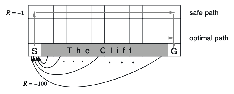
The action space consists of 4 movement: up, down, right, and left. Reward is \(−1\) on all transitions except stepping into the the cliff region, which incurs a reward of \(−100\) and sends the agent instantly back to the start.

A possible implementation:

class CliffWalkingEnv:
    def __init__(self, ncol, nrow):
        self.nrow = nrow
        self.ncol = ncol
        
        # At the initial state S.
        self.x = 0
        self.y = self.nrow - 1
	
    def step(self, action):
		"""One step the agent can take."""
        # change[0]:up, change[1]:down, change[2]:left, change[3]:right
        change = [[0, -1], [0, 1], [-1, 0], [1, 0]]
        
        # position after taking the action
        self.x = min(self.ncol - 1, max(0, self.x + change[action][0]))
        self.y = min(self.nrow - 1, max(0, self.y + change[action][1]))
        
        # flatterned serial number of the current state
        next_state = self.y * self.ncol + self.x
        reward = -1
        done = False
        
        # current location is at the cliff or the target
        if self.y == self.nrow - 1 and self.x > 0:  
            done = True
            # current location is at the cliff
            if self.x != self.ncol - 1:
                reward = -100
        
        return next_state, reward, done
	
    def reset(self):
	    """Return to the initial state."""
        self.x = 0
        self.y = self.nrow - 1
        return self.y * self.ncol + self.x

Experiments are conducted in Google Colab.

References

[1] Richard S. Sutton, Andrew G. Barto. (2014). Reinforcement Learning: An Introduction. The MIT Press.

[2] Watkins, C. J., Dayan, P. (1992). Technical Note: Q-learning. Machine learning, 8(3-4), 279-292.

[3] Aston Zhang, Zachary C. Lipton, Mu Li, Alexander J. Smola. (2023). Dive into Deep Learning. Cambridge University Press.