Overview

在现代机器学习的应用中，分类问题无处不在。从电子邮件的垃圾分类到肿瘤的良恶性判断，从图像目标检测到语音情感分析，分类算法为各领域提供了强大的工具。然而，针对分类问题，不同算法在模型假设、适用数据特性以及分类效果上表现各异。

生成式学习和判别式学习是分类问题中两种主要的算法框架。生成式学习通过建模数据的生成过程，捕捉输入特征和类别之间的联合分布，以高斯判别分析为代表，擅长处理输入特征服从高斯分布的连续型数据；而判别式学习则直接学习类别的决策边界，逻辑回归是其典型方法，以其灵活性和鲁棒性在多种复杂场景中得到广泛应用。

本文聚焦于高斯判别分析与逻辑回归在分类问题中的应用，从理论框架、模型假设和算法优势出发，探讨两者在不同场景下的表现和局限性。

逻辑回归 (Logistic Regression)

与线性回归问题类似，对于一个二元分类问题，我们希望预测的值 $y$ 只能取两个离散的值，即 $0$ 和 $1$ 。举个例子，如果我们想建立一个电子邮件的垃圾邮件分类器，输入 $x_i$ 可能是一封邮件的某些特征，输出的对应标签 $y_i$ 则可能是1(表示垃圾邮件)或0(表示非垃圾邮件)。

由于预测值 $y$ 满足 $y∈\{0, 1\}$，如果我们直接使用线性回归的假设函数 $h_θ(x)=θ^T x$，当 $h_θ(x)$ 大于 $1$ 或小于 $0$ 时，该假设函数失去了合理性。为了解决这个问题，我们改变假设函数的形式，令

$$ h_\theta\left(x\right)=sigmoid\left(\theta^Tx\right)=\frac{1}{1+e^{-\theta^{T}x}} $$

其中，$sigmoid: g\left(z\right)=\frac{1}{1+e^{-z}}$ ，又称S型生长曲线，值域为 $(0, 1)$。

根据以上假设，我们可以发现，模型仅有 $θ$ 这一个参数，我们通过最大似然估计拟合该参数。

我们可以假设标签 $y$ 由伯努利分布生成，即：

$$ P\left(y=1\vert x;\theta\right)=h_\theta\left(x\right) $$$$ P\left(y=0\vert x;\theta\right)=1-h_\theta\left(x\right) $$

为了后续推导可以写成：

$$ P\left(y\vert x;\theta\right)=\left(h_\theta\left(x\right)\right)^y\left(1-h_\theta\left(x\right)\right)^{1-y} $$

我们假设训练样本独立同分布，则数据的似然函数为：

$$ \mathcal{L}\left(\theta\right)=\prod_{i=1}^{m}{p\left(y^{\left(i\right)}\vert x^{\left(i\right)};\theta\right)}=\prod_{i=1}^{m}{\left(h_\theta\left(x^{\left(i\right)}\right)\right)^{y^{\left(i\right)}}\left(1-h_\theta\left(x^{\left(i\right)}\right)\right)^{1-y^{\left(i\right)}}} $$

对数似然函数为：

$$ \ell\left(\theta\right)=\sum_{i=1}^{m}\left(y^{\left(i\right)}log{h_\theta}\left(x^{\left(i\right)}\right)+\left(1-y^{\left(i\right)}\right)log{\left(1-h_\theta\left(x^{\left(i\right)}\right)\right)}\right) $$

我们通过梯度上升法最大化对数似然函数。对于单个训练样本(x, y)，梯度计算如下：

$$ \begin{equation} \begin{aligned} \frac{\partial}{\partial\theta_j}\ell\left(\theta\right)&=\frac{\partial}{\partial\theta_j}\sum_{i=1}^{m}\left(y^{\left(i\right)}\log{h_\theta}\left(x^{\left(i\right)}\right)+\left(1-y^{\left(i\right)}\right)\log{\left(1-h_\theta\left(x^{\left(i\right)}\right)\right)}\right) \\ &=\sum_{i=1}^{m}y^{\left(i\right)}\frac{\partial}{\partial\theta_j}\log{h_\theta}\left(x^{\left(i\right)}\right)+\sum_{i=1}^{m}{\left(1-y^{\left(i\right)}\right)\frac{\partial}{\partial\theta_j}\log{\left(1-h_\theta\left(x^{\left(i\right)}\right)\right)}} \end{aligned} \end{equation} $$

注意到 $sigmoid$ 函数存在性质：

$$ g^\prime\left(z\right)=g\left(z\right)\left(1-g\left(z\right)\right) $$

故有：

$$ \begin{equation} \begin{aligned} \frac{\partial}{\partial\theta_j}\log{h_\theta}\left(x^{\left(i\right)}\right) &= \frac{h_\theta\left(x^{\left(i\right)}\right)\left(1-h_\theta\left(x^{\left(i\right)}\right)\right)x_j}{h_\theta\left(x^{\left(i\right)}\right)} \\ &= \left(1-h_\theta\left(x^{\left(i\right)}\right)\right)x_j \end{aligned} \end{equation} $$$$ \begin{equation} \begin{aligned} \frac{\partial}{\partial\theta_j}\log\left(1-h_\theta\left(x^{(i)}\right)\right) &= \frac{-h_\theta\left(x^{(i)}\right)\left(1-h_\theta\left(x^{(i)}\right)\right)x_j}{1-h_\theta\left(x^{(i)}\right)} \\ &= -h_\theta\left(x^{(i)}\right)x_j \end{aligned} \end{equation} $$

代入原式：

$$ \begin{equation} \begin{aligned} \frac{\partial}{\partial\theta_j}\ell\left(\theta\right) &= \sum_{i=1}^{m}{y^{\left(i\right)}\left(1-h_\theta\left(x^{\left(i\right)}\right)\right)x_j-\sum_{i=1}^{m}\left(1-y^{\left(i\right)}\right)}h_\theta\left(x^{\left(i\right)}\right)x_j \\ &= \sum_{i=1}^{m}{\left(y^{\left(i\right)}-h_\theta\left(x^{\left(i\right)}\right)\right)x_j} \end{aligned} \end{equation} $$

因此，随机梯度上升的更新规则为：

$$ \theta_j≔θj+α(y^{(i)}-h_θ(x^{(i)}))x_j^{(i)} $$

其中，$α$ 为学习率，可人为控制。

生成式学习算法 (Generative Learning algorithms)

在介绍高斯判别分析前，我们先简单了解一下生成式学习算法。假设我们有一个分类问题，给定一个训练集，希望通过某些动物的特征学习如何区分猫 $(y=0)$ 和狗 $(y=1)$。如果应用逻辑回归算法，基本思路是尝试找到一个多维空间的超平面，即一个决策边界，用于分隔这两种动物。然后，对于一个新动物，算法检查它落在哪边，以此进行预测。而生成式学习算法的基本思路是：首先，针对猫，我们可以构建一个模型来描述猫的特征。同样地，我们为狗构建一个单独的模型。最后，为了分类一个新动物，我们将新动物与猫的模型进行匹配，也与狗的模型进行匹配，看看它更像训练集中出现的猫还是狗。

可见，生成式学习算法的核心目标是建模输入数据 $x$ 在给定标签 $y$ 下的条件分布 $p(x\vert y)$，以及标签的先验分布 $p(y)$。带入上面的情境，$p(x\vert y)=0$ 建模了猫的特征分布，而 $p(x\vert y)=1$ 建模了狗的特征分布。这一方法通过全面建模数据的生成机制，为预测问题提供了一种概率论基础。利用贝叶斯公式，生成式算法能够根据后验分布 $p(y\vert x)$ 进行预测:

$$ p\left(y\middle|\ x\right)=\frac{p\left(x\middle|\ y\right)p\left(y\right)}{p\left(x\right)} $$

其中，$p(x)$ 可通过 $\ p\left(x\right)=\sum\limits_{y}{\left(x\middle\vert\ y\right)p\left(y\right)}$ 进行计算。而实际上，由于

$$ \arg\max\limits _y p\left(y\middle\vert\ x\right)=\arg\max\limits _y p \left(x\middle\vert\ y\right)p\left(y\right) $$

在进行预测即最大化 $p(y\vert x)$ 时，我们并不需要真正计算分母。

高斯判别分析 (Gaussian Discriminant Analysis, GDA)

GDA是一种典型的生成式学习算法，适用于输入特征 $x$ 是连续型随机变量的分类问题。我们先提出该模型的建模假设如下。

GDA假设标签y由伯努利分布生成，即

$$ y\sim B(1,ϕ) $$

根据伯努利分布的定义，可知

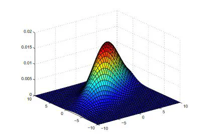
$$ P(y=1)=ϕ $$$$ P(y=0)=1-ϕ $$

GDA假设 $p(x\vert y)$ 的条件分布是多元高斯分布，这一假设为模型提供了明确的数学框架。在给定 $y=0$ 或 $y=1$ 的条件下，输入特征 $x$ 分别服从两个不同的多元高斯分布，即

$$ x\vert y=0\sim N(μ_0,Σ) $$$$ x\vert y=1\sim N(μ_1,Σ) $$

根据多元高斯分布的定义，可知

$$ p\left(x\middle|\ y=0\right)=\frac{1}{\left(2\pi\right)^\frac{d}{2}\left|\Sigma\right|^\frac{1}{2}}exp{\left(-\frac{1}{2}\left(x-\mu_0\right)^T\Sigma^{-1}\left(x-\mu_0\right)\right)} $$$$ p\left(x\middle|\ y=1\right)=\frac{1}{\left(2\pi\right)^\frac{d}{2}\left|\Sigma\right|^\frac{1}{2}}exp{\left(-\frac{1}{2}\left(x-\mu_1\right)^T\Sigma^{-1}\left(x-\mu_1\right)\right)} $$

根据以上两个假设，我们可以发现，该模型共有 $ϕ,Σ,μ_0,μ_1$ 四个参数。尽管对于不同的标签 $y$，我们有不同的均值向量，但在模型的实际应用中，通常使用同一个协方差矩阵 $Σ$。下面，我们使用最大似然估计来推导这四个参数。

数据的对数似然函数为：

$$ \ell\left(\phi,\mu_0,\mu_1,\Sigma\right)=log{\prod_{i=1}^{n}p\left(x^{\left(i\right)},y^{\left(i\right)};\phi,\mu_0,\mu_1,\Sigma\right)} $$

通过求该函数的梯度向量，可得四个参数的最大似然估计为：

$$ \phi=\frac{1}{n}\sum_{i=1}^{n}y^{\left(i\right)} $$$$ \mu_0=\frac{\sum\limits_{i=1}^{n}{x^{\left(i\right)} \{y^{\left(i\right)}=0\}}}{\sum\limits_{i=1}^{n_0}{1 \{y^{\left(i\right)}=0\}}} $$$$ \mu_1=\frac{\sum_{i=1}^{n}{x^{\left(i\right)} \{y^{\left(i\right)}=1\}}}{\sum_{i=1}^{n_1}{1 \{y^{\left(i\right)}=1\}}} $$$$ \Sigma=\frac{1}{n}\sum_{i=1}^{n}{\left(x^{\left(i\right)}-\mu_{y^{\left(i\right)}}\right)\left(x^{\left(i\right)}-\mu_{y^{\left(i\right)}}\right)^T} $$

具体推导过程如下：

$$ \begin{equation} \begin{aligned} \ell\left(\phi,\mu_0,\mu_1,\Sigma\right) &= \log{\prod_{i=1}^{n}p\left(x^{\left(i\right)},y^{\left(i\right)};\phi,\mu_0,\mu_1,\Sigma\right)} \\ &= \log{\prod_{i=1}^{n}p\left(x^{\left(i\right)}|y^{\left(i\right)};\mu_0,\mu_1,\Sigma\right)p\left(y^{\left(i\right)};\phi\right)} \\ &= \sum_{i=1}^{n}{\log{p}\left(x^{\left(i\right)}\middle|\ y^{\left(i\right)};\mu_0,\mu_1,\Sigma\right)+\sum_{i=1}^{n}{\log{p}\left(y^{\left(i\right)};\phi\right)}} \end{aligned} \end{equation} $$

• 对于参数 $\phi$

$$ \begin{equation} \begin{aligned} \frac{\partial\ell}{\partial\phi} &= 0+\frac{\partial}{\partial\phi}\sum_{i=1}^{n}{log{\phi^{y^{\left(i\right)}}}\left(1-\phi\right)^{\left(1-y^{\left(i\right)}\right)}} \\ &= \frac{\partial}{\partial\phi}\left(log{\phi\sum_{i=1}^{n}y^{\left(i\right)}}+log{\left(1-\phi\right)}\sum_{i=1}^{n}\left(1-y^{\left(i\right)}\right)\right) \\ &= \frac{1}{\phi}\sum_{i=1}^{n}y^{\left(i\right)}+\frac{1}{\phi-1}\left(n-\sum_{i=1}^{n}y^{\left(i\right)}\right) \end{aligned} \end{equation} $$

令 $\frac{\partial\ell}{\partial\phi}=0$ ，可得：

$$ \phi=\frac{1}{n}\sum_{i=1}^{n}y^{\left(i\right)} $$

• 对于参数 $\mu_0$

$$ \begin{equation} \begin{aligned} \frac{\partial\ell}{\partial\mu_0} &= \frac{\partial}{\partial\mu_0}\sum_{i=1}^{n}log{\frac{exp{\left(-\frac{1}{2}\left(x^{\left(i\right)}-\mu_0\right)^T\Sigma^{-1}\left(x^{\left(i\right)}-\mu_0\right)\right)}}{\left(2\pi\right)^\frac{d}{2}\left|\Sigma\right|^\frac{1}{2}}} \\ &= \frac{\partial}{\partial\mu_0}\sum_{i=1}^{n}\left[-\frac{1}{2}\left(x^{\left(i\right)}-\mu_0\right)^T\Sigma^{-1}\left(x^{\left(i\right)}-\mu_0\right)\right] \\ &= -\frac{1}{2}\sum_{i=1}^{n}\frac{\partial}{\partial (x^{\left(i\right)}-\mu_0)}\left[\left(x^{\left(i\right)}-\mu_0\right)^T\Sigma^{-1}\left(x^{\left(i\right)}-\mu_0\right)\right] \\ &= -\frac{1}{2}\sum_{i=1}^{n}\left[\Sigma^{-1}+\left(\Sigma^{-1}\right)^T\right]\left(\mu_0-x^{\left(i\right)}\right) \\ &= -\frac{1}{2}\left[\Sigma^{-1}+\left(\Sigma^{-1}\right)^T\right]\left(n\mu_0-\sum_{i=1}^{n}x^{\left(i\right)}\right) \end{aligned} \end{equation} $$

令 $\frac{\partial\ell}{\partial\mu_0}=0$，可得：

$$ \mu_0=\frac{\sum\limits_{i=1}^{n}{x^{\left(i\right)} \{y^{\left(i\right)}=0\}}}{\sum\limits_{i=1}^{n}{1\ \{y^{\left(i\right)}=0\}}} $$

• 对于参数 $\mu_1$，同理可得:

$$ \mu_1=\frac{\sum\limits_{i=1}^{n}{x^{\left(i\right)} \{y^{\left(i\right)}=1\}}}{\sum\limits_{i=1}^{n}{1\ \{y^{\left(i\right)}=1\}}} $$

• 对于参数 $\Sigma$

$$ \frac{\partial\ell}{\partial\Sigma}=\frac{\partial}{\partial\Sigma}\left(ln{\left|\Sigma\right|+\frac{1}{n}\sum_{i=1}^{n}{\left(x^{\left(i\right)}-\mu_{y^{\left(i\right)}}\right)^T\Sigma^{-1}\left(x^{\left(i\right)}-\mu_{y^{\left(i\right)}}\right)}}\right) $$

前一部分

$$ \begin{equation} \begin{aligned} \mathrm{d}\mathrm{ln}{\left|\mathrm{\Sigma}\right|} &= \left|\Sigma\right|^{-1}\mathrm{\mathrm{d}}\left|\Sigma\right| \\ &= \left|\Sigma\right|^{-1}\left|\Sigma\right|\mathrm{\mathrm{tr}}\left(\mathrm{\Sigma}^{\mathrm{-1}}\mathrm{d\Sigma} \right) \\ &= \mathrm{\mathrm{tr}}\left(\mathrm{\Sigma}^{\mathrm{-1}}\mathrm{d\Sigma} \right) \end{aligned} \end{equation} $$

后一部分

$$ \begin{equation} \begin{aligned} & \mathrm{d}\left[\frac{\mathrm{1}}{\mathrm{n}}\sum_{\mathrm{i=1}}^{\mathrm{n}}{\left(\mathrm{x}^{\left(\mathrm{i}\right)}\mathrm{-}\ \mathrm{\mu}_{\mathrm{y}^{\left(\mathrm{i}\right)}}\right)^\mathrm{T}\mathrm{\Sigma}^{\mathrm{-1}}\left(\mathrm{x}^{\left(\mathrm{i}\right)}\mathrm{-}\ \mathrm{\mu}_{\mathrm{y}^{\left(\mathrm{i}\right)}}\right)}\right] \\ &= \frac{\mathrm{1}}{\mathrm{n}}\sum_{\mathrm{i=1}}^{\mathrm{n}}{\left(\mathrm{x}^{\left(\mathrm{i}\right)}\mathrm{-}\ \mathrm{\mu}_{\mathrm{y}^{\left(\mathrm{i}\right)}}\right)^\mathrm{T}{\mathrm{d(\Sigma}}^{\mathrm{-1}})\left(\mathrm{x}^{\left(\mathrm{i}\right)}\mathrm{-}\ \mathrm{\mu}_{\mathrm{y}^{\left(\mathrm{i}\right)}}\right)} \\ &= \frac{\mathrm{1}}{\mathrm{n}}\sum_{\mathrm{i=1}}^{\mathrm{n}}{\left(\mathrm{x}^{\left(\mathrm{i}\right)}\mathrm{-}\ \mathrm{\mu}_{\mathrm{y}^{\left(\mathrm{i}\right)}}\right)^\mathrm{T}{\mathrm{\Sigma}^{\mathrm{-1}}\mathrm{d(\Sigma)\Sigma}\ }^{\mathrm{-1}}\left(\mathrm{x}^{\left(\mathrm{i}\right)}\mathrm{-}\ \mathrm{\mu}_{\mathrm{y}^{\left(\mathrm{i}\right)}}\right)} \\ &= \frac{\mathrm{1}}{\mathrm{n}}\sum_{\mathrm{i=1}}^{\mathrm{n}}\mathrm{tr}\left(\left(\mathrm{x}^{\left(\mathrm{i}\right)}\mathrm{-}\ \mathrm{\mu}_{\mathrm{y}^{\left(\mathrm{i}\right)}}\right)^\mathrm{T}{\mathrm{\Sigma}^{\mathrm{-1}}\mathrm{d(\Sigma)\Sigma}\ }^{\mathrm{-1}}\left(\mathrm{x}^{\left(\mathrm{i}\right)}\mathrm{-}\ \mathrm{\mu}_{\mathrm{y}^{\left(\mathrm{i}\right)}}\right)\right) \\ &= \frac{\mathrm{1}}{\mathrm{n}}\sum_{i=1}^{n}\mathrm{tr}\left(\mathrm{\Sigma}^{\mathrm{-1}}\left(\mathrm{x}^{\left(\mathrm{i}\right)}\mathrm{-}\ \mathrm{\mu}_{\mathrm{y}^{\left(\mathrm{i}\right)}}\right)\left(\mathrm{x}^{\left(\mathrm{i}\right)}\mathrm{-}\ \mathrm{\mu}_{\mathrm{y}^{\left(\mathrm{i}\right)}}\right)^\mathrm{T}\mathrm{\Sigma}^{\mathrm{-1}}\mathrm{d\Sigma}\ \right) \\ &= \mathrm{\mathrm{tr}}\left(\left(-\frac{\mathrm{1}}{\mathrm{n}}\right)\mathrm{\Sigma}^{\mathrm{-1}}\left(\sum_{i=1}^{n}{\left(\mathrm{x}^{\left(\mathrm{i}\right)}\mathrm{-} \mathrm{\mu}_{\mathrm{y}^{\left(\mathrm{i}\right)}}\right)\left(\mathrm{x}^{\left(\mathrm{i}\right)}\mathrm{-} \mathrm{\mu}_{\mathrm{y}^{\left(\mathrm{i}\right)}}\right)^\mathrm{T}}\right)\mathrm{\Sigma}^{\mathrm{-1}}\mathrm{d\Sigma} \right) \end{aligned} \end{equation} $$

故

$$ \begin{equation} \begin{aligned} & \mathrm{d}\mathrm{ln}{\left|\mathrm{\Sigma}\right|}+\mathrm{\mathrm{d}}\left[\frac{1}{\mathrm{n}}\sum_{\mathrm{i=1}}^{\mathrm{n}}{\left(\mathrm{x}^{\left(\mathrm{i}\right)}\mathrm{-} \mathrm{\mu}_{\mathrm{y}^{\left(\mathrm{i}\right)}}\right)^\mathrm{T}\mathrm{\Sigma}^{\mathrm{-1}}\left(\mathrm{x}^{\left(\mathrm{i}\right)}\mathrm{-} \mathrm{\mu}_{\mathrm{y}^{\left(\mathrm{i}\right)}}\right)}\right] \\ &= \mathrm{\mathrm{tr}}\left(\left(\mathrm{\Sigma}^{\mathrm{-1}}-\mathrm{\Sigma}^{\mathrm{-1}}\frac{\mathrm{1}\ }{\mathrm{n}}\left(\sum_{i=1}^{n}{\left(\mathrm{x}^{\left(\mathrm{i}\right)}\mathrm{-}\ \mathrm{\mu}_{\mathrm{y}^{\left(\mathrm{i}\right)}}\right)\left(\mathrm{x}^{\left(\mathrm{i}\right)}\mathrm{-}\ \mathrm{\mu}_{\mathrm{y}^{\left(\mathrm{i}\right)}}\right)^\mathrm{T}}\right)\mathrm{\Sigma}^{\mathrm{-1}}\right)\mathrm{d\Sigma} \right) \end{aligned} \end{equation} $$

即

$$ \frac{\partial\ell}{\partial\Sigma}=\left(\mathrm{\Sigma}^{\mathrm{-1}}-\mathrm{\Sigma}^{\mathrm{-1}}\frac{\mathrm{1}\ }{\mathrm{n}}\left(\sum_{i=1}^{n}{\left(\mathrm{x}^{\left(\mathrm{i}\right)}\mathrm{-}\ \mathrm{\mu}_{\mathrm{y}^{\left(\mathrm{i}\right)}}\right)\left(\mathrm{x}^{\left(\mathrm{i}\right)}\mathrm{-}\ \mathrm{\mu}_{\mathrm{y}^{\left(\mathrm{i}\right)}}\right)^\mathrm{T}}\right)\mathrm{\Sigma}^{\mathrm{-1}}\right)^T $$

令 $\frac{\partial\ell}{\partial\Sigma}=0$，可得：

$$ \Sigma=\frac{1}{n}\sum_{i=1}^{n}{\left(x^{\left(i\right)}-\mu_{y^{\left(i\right)}}\right)\left(x^{\left(i\right)}-\mu_{y^{\left(i\right)}}\right)^T} $$

高斯判别分析与逻辑回归的区别

GDA模型和逻辑回归模型存在一个有趣的关系。如果我们将 $p(y=1\vert x;ϕ,μ0,μ1,Σ0)$ 视作 $x$ 的函数，可以发现它可以被表达为以下的形式：

$$ p\left(y=1\middle|\ x;\phi,\mu_0,\mu_1,\Sigma\right)=\frac{1}{1+\exp{\left(-\theta^Tx\right)}}=sigmoid\left(\theta^Tx\right) $$

具体推导如下：

由多元高斯分布定义可知

$$ p\left(x\middle|\ y=0\right)=\frac{1}{\left(2\pi\right)^\frac{d}{2}\left|\Sigma\right|^\frac{1}{2}}\exp{\left(-\frac{1}{2}\left(x-\mu_0\right)^T\Sigma^{-1}\left(x-\mu_0\right)\right)} $$$$ p\left(x\middle|\ y=1\right)=\frac{1}{\left(2\pi\right)^\frac{d}{2}\left|\Sigma\right|^\frac{1}{2}}\exp{\left(-\frac{1}{2}\left(x-\mu_1\right)^T\Sigma^{-1}\left(x-\mu_1\right)\right)} $$

由贝叶斯公式

$$ \begin{equation} \begin{aligned} p\left(y=1\middle|\ x\right) &= \frac{p\left(x\middle|\ y=1\right)p\left(y=1\right)}{p\left(x\middle|\ y=1\right)p\left(y=1\right)+p\left(x\middle|\ y=0\right)p\left(y=0\right)} \\ &= \frac{\phi\exp{\left(-\frac{1}{2}\left(x-\mu_1\right)^T\Sigma^{-1}\left(x-\mu_1\right)\right)}}{\phi\exp{\left(-\frac{1}{2}\left(x-\mu_1\right)^T\Sigma^{-1}\left(x-\mu_1\right)\right)+\left(1-\phi\right)\exp{\left(-\frac{1}{2}\left(x-\mu_0\right)^T\Sigma^{-1}\left(x-\mu_0\right)\right)}}} \\ &= \frac{1}{1+\frac{1-\phi}{\phi}\exp{\left(-\frac{1}{2}[\left(x-\mu_0\right)^T\Sigma^{-1}\left(x-\mu_0\right)-\left(x-\mu_1\right)^T\Sigma^{-1}\left(x-\mu_1\right)]\right)}} \\ &= \frac{1}{1+\frac{1-\phi}{\phi}\exp{\left(-\frac{1}{2}\left[2\left(\mu_1-\mu_0\right)^T{\ \Sigma}^{-1}x-\left(\mu_1^T{\Sigma^{-1}\mu}_1-\mu_0^T\Sigma^{-1}\mu_0\right)\right]\right)}} \\ &= \frac{1}{1+\exp{\left(-\left(\mu_1-\mu_0\right)^T{\ \Sigma}^{-1}x+\frac{1}{2}\left(\mu_1^T{\Sigma^{-1}\mu}_1-\mu_0^T\Sigma^{-1}\mu_0\right)+log{\left(\frac{1-\phi}{\phi}\right)}\right)}} \end{aligned} \end{equation} $$

不难发现指数中为关于 $x$ 的线性函数，故一定可以写成：

$$ \frac{1}{1+exp{\left(-\theta^Tx\right)}} $$

可见，如果 $x\vert y$ 服从多元高斯分布(共享协方差矩阵 $Σ$)，那么 $p(y\vert x)$ 必然可以写成逻辑函数形式。然而反之则不成立，即使 $p(y\vert x)$ 是逻辑函数形式，也无法保证 $p(x\vert y)$ 是多元高斯分布。

这表明，GDA模型对数据的建模假设比逻辑回归更为强烈，具体体现在对条件分布 $p(x\vert y)$ 和共享协方差矩阵 $Σ$ 的高斯分布假设上。当这些假设与数据实际分布一致时，GDA 能够充分利用这些信息进行参数估计，因此在描述数据生成机制和预测准确性方面表现出显著优势。特别是，当 $p(x\vert y)$ 确实是多元高斯分布(共享 $Σ$)时，GDA 被证明是渐近有效的，即随着训练集规模的增大，没有任何其他算法能在估计后验概率 $p(y\vert x)$ 的准确性上超过GDA。在大样本情况下，这种优势尤其显著，使得GDA成为符合建模假设时的最佳选择。

相比之下，逻辑回归对数据分布假设的依赖较弱，因此在模型的灵活性和对噪声的鲁棒性上更具优势。逻辑回归不需要假设 $p(x\vert y)$ 的具体形式，只需直接建模 $p(y\vert x)$ 为逻辑函数。这使得逻辑回归能够适应各种数据分布。例如，即便 $x\vert y=0\sim P(λ_0)$，且 $x\vert y=1\sim P(λ_1)$ 分别服从非高斯的泊松分布，后验概率 $p(y\vert x)$ 依然可以用逻辑函数表示，从而保证逻辑回归模型的有效性和稳健性。

然而，当数据分布偏离高斯假设时，GDA的性能则可能受到显著影响。此时，强行用高斯分布拟合可能导致分类边界的不准确，甚至模型无法很好地捕捉数据的真实规律，表现出不可预测的效果。这种情况下，逻辑回归的灵活性反而使其在非高斯数据场景中表现更为稳定和可靠。总的来说，两者在分类问题中的适用性取决于具体数据的分布特性和建模需求，对于数据分布信息明确且符合高斯假设的问题，GDA 是优选；而对于数据分布未知或复杂多样的情况，逻辑回归往往能提供更为稳健的解决方案。

参考文献

[1] Sergios Theodoridis. 机器学习：贝叶斯和优化方法[M]. 机械工业出版社，2022-2.

[2] Trevor Hastie. Discriminant Analysis by Gaussian Mixtures[J]. Journal of the Royal Statistical Society: Series B (Methodological), Volume 58, Issue 1, January 1996, Pages 155–176.

[3] Jie Gui. A Review on Generative Adversarial Networks: Algorithms, Theory, and Applications[J]. IEEE Transactions on Knowledge and Data Engineering (Volume: 35, Issue: 4, 01 April 2023, Pages: 3313 - 3332)