I think blogging about my first time digging into reinforcement learning (RL) theory would be fun. So boom, here it goes!

This post begins with the classic Markov decision process (MDP) formulation, moves through dynamic programming and Monte Carlo Methods, and then uses those ideas to arrive at temporal-difference learning.

Markov Decision Processes

Problem Framing

The reinforcement learning (RL) problem is meant to be a straightforward framing of the problem of learning from interaction to achieve a goal, or more vividly, “trial and error”.

The learner and decision-maker is called the agent. The thing it interacts with, comprising everything outside the agent, is called the environment. These two interact at each of a sequence of discrete time steps, $t=0,1,2,3,\dots$. At each time step $t$, the agent receives some representation of the environment’s state, $S_t\in\mathcal{S}$, where $\mathcal{S}$ is the set of possible states, and on that basis selects an action, $A_t\in\mathcal{A}(S_t)$, where $\mathcal{A}(S_t)$ is the set of actions available in state $S_t$. One time step later, in part as a consequence of its action, the agent receives a numerical reward, $R_{t+1}\in\mathcal{R}\subset\mathbb{R}$, and finds itself in a new state, $S_{t+1}$.

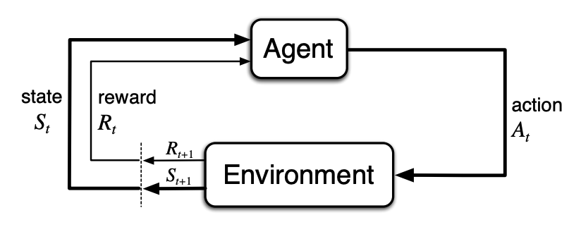
Consider the situation when the system starts at a particular state $S_t\in\mathcal{S}$ and continuously taking actions after time step $t$, resulting in a trajectory like

\[\begin{equation} \tau=(S_t,A_t,R_{t+1},S_{t+1},A_{t+1},R_{t+2},S_{t+2},A_{t+2},R_{t+3},\dots). \end{equation}\]

In general, we seek to maximize the expected return, where $G_t$ can be defined in the simplest case as the cumulative reward the agent receives after time step $t$:

\[\begin{equation} G_t=R_{t+1}+R_{t+2}+R_{t+3}+\cdots+R_T, \end{equation}\]

where $T$ is the final time step.

Since this expected return will be infinite when $T=\infty$, the learning process above would possibly fail. In order to prevent this from happening, we introduce a parameter called the discount rate $0\leq\gamma\leq 1$ to (1) as:

\[\begin{equation} G_t = R_{t+1} + \gamma R_{t+2} + \gamma^2 R_{t+3}+\cdots = \sum\limits_{k=0}^\infty\gamma^k R_{t+k+1}. \end{equation}\]

If $\gamma<1$, the infinite sum has a finite value as long as the reward sequence ${R_k}$ is bounded. If $\gamma=0$, the agent is “myopic” in being concerned only with maximizing immediate rewards. As $\gamma$ approaches $1$, the objective takes future rewards into account more strongly: the agent becomes more farsighted.

The Markov Property

In the RL framework, the agent makes its decisions as a function of a signal from the environment’s state. In broad sense, “the state” means whatever information that is available to the agent. And we expect the state satisfies the Markov property, which we defined as follow.

Consider the response given by a general environment at time ${t+1}$ to the action taken at time $t$, which may depend on everything that has happened earlier. In this case the dynamics can be defined as:

\[\begin{equation} \Pr\{S_{t+1}=s^\prime, R_{t+1}=r \vert S_0,A_0,R_1,\dots,S_{t-1},A_{t-1},R_t,S_t,A_t\}, \end{equation}\]

for all possible $r$ and $s^\prime$. If the environment’s response at $t+1$ depends only on the state and action representations at $t$, i.e.

\[\begin{equation} p(s^\prime, r \vert s,a)=\Pr\{S_{t+1}=s^\prime, R_{t+1}=r \vert S_t,A_t\}, \end{equation}\]

for all $s^\prime,r,S_t,A_t$, we say the state signal has the Markov property and is a Markov state.

A reinforcement learning task that satisfies the Markov property is called a Markov decision process (MDP), which models how a system changes state when different actions are applied. Formally, given any state $s$ and action $a$, the dynamics of an MDP can be specified by:

\[\begin{equation} p(s^\prime, r \vert s,a)=\Pr\{S_{t+1}=s^\prime, R_{t+1}=r \vert S_t=s,A_t=a\}. \end{equation}\]

Value Functions

The value function of a state (or state-action pair) estimates how good or bad an individual is in a given state (or how good it is to perform a given action in a given state). And the notion of “how good” here is defined in terms of expected returns when starting in a specific state and following a specific behavior thereafter. Formally, we call this kind of behavior as a policy, $\pi(a\vert s)$, which is a conditional distribution over the actions $a\in\mathcal{A}$ given the state $s\in\mathcal{S}$.

For MDPs, we can define the value of a state $s$ under a policy $\pi$ as

\[\begin{equation} v_\pi(s) = \mathbb{E}_\pi\left[G_t\vert S_t=s\right] = \mathbb{E}_\pi\left[\left.\sum_{k=0}^{\infty}\gamma^k R_{t+k+1}\right\vert S_t=s\right], \end{equation}\]

where $\mathbb{E}\pi$ denotes the expected value of a random variable given that the agent follows policy $\pi$, and $t$ is any time step. The function $v\pi$ is called the state-value function for policy $\pi$.

Similarly, we define the value of taking action $a$ in state $s$ under a policy $\pi$ as

\[\begin{equation} q_\pi(s,a) =\mathbb{E}_\pi\left[G_t\vert S_t=s,A_t=a\right] = \mathbb{E}_\pi\left[\left.\sum_{k=0}^{\infty}\gamma^k R_{t+k+1}\right\vert S_t=s,A_t=a\right]. \end{equation}\]

The function $q_\pi$ is called the action-value function for policy $\pi$.

A fundamental property of value functions is that they satisfy particular recursive relationships. The value function can be mathematically decomposed into

\[\begin{equation} \begin{align*} v_\pi(s) &= \mathbb{E}_\pi\left[\left.\sum_{k=0}^{\infty}\gamma^k R_{t+k+1}\right\vert S_t=s\right] \\ &= \mathbb{E}_\pi\left[\left. R_{t+1}+\gamma\sum_{k=0}^{\infty}\gamma^k R_{t+k+2}\right\vert S_t=s\right] \\ &= \sum_{a\in\mathcal{A}(s)} \pi(a\vert s)\sum_{s^\prime\in\mathcal{S}}\sum_{r\in\mathcal{R}} p(s^\prime,r\vert s, a) \left[ r + \gamma\mathbb{E}_\pi\left[\left.\sum_{k=0}^{\infty}\gamma^k R_{t+k+2}\right\vert S_{t+1}=s^\prime\right]\right] \\ &= \sum_{a\in\mathcal{A}(s)} \pi(a\vert s)\sum_{s^\prime\in\mathcal{S}}\sum_{r\in\mathcal{R}} p(s^\prime,r\vert s, a) \left[r + \gamma v_\pi(s^\prime)\right], \\ \end{align*} \end{equation}\]

which is the foundation of dynamic programming upon which all RL algorithms are based. This is the Bellman equation for $v_\pi$, which expresses a relationship between the value of the state and the values of its successor state.

Optimal Policy

Solving a RL task roughly means finding an optimal policy $\pi^*$ that maximize the expected return, which shares the same state-value function

\[\begin{equation} v^*(s)=\max_\pi v_\pi(s),\quad \forall s\in\mathcal{S} \end{equation}\]

and the same action value function

\[\begin{equation} q^*(s,a)=\max_\pi q_\pi(s,a),\quad \forall s\in\mathcal{S},a\in\mathcal{A}(s). \end{equation}\]

Intuitively, the value of a state under an optimal policy must equal the expected return for the best action from that state. Starting from this fact, we can derive the so-called Bellman optimality equation for $v^*$:

\[\begin{equation} \begin{align*} v^*(s) &= \max_{a\in\mathcal{A}(s)}q_{\pi_*}(s,a) \\ &= \max_{a\in\mathcal{A}(s)}\mathbb{E}_{\pi^*}\left[\left.\sum_{k=0}^{\infty}\gamma^k R_{t+k+1}\right\vert S_t=s,A_t=a\right] \\ &= \max_{a\in\mathcal{A}(s)}\mathbb{E}_{\pi^*}\left[R_{t+1}+\left.\gamma\sum_{k=0}^{\infty}\gamma^k R_{t+k+2}\right\vert S_t=s,A_t=a\right] \\ &= \max_{a\in\mathcal{A}(s)}\mathbb{E}_{\pi^*}\left[R_{t+1}+\left.\gamma v^*(S_{t+1})\right\vert S_t=s,A_t=a\right] \\ &= \max_{a\in\mathcal{A}(s)}\sum_{s^\prime,r} p(s^\prime,r\vert s,a)[r+\gamma v^*(s^\prime)]. \end{align*} \end{equation}\]

Similarly, we can also derive the Bellman optimality equation for $q^*$ is

\[\begin{equation} \begin{align*} q^*(s,a) &= \mathbb{E}_{\pi^*}\left[\left.R_{t+1}+\gamma\max_{a^\prime} q^*(S_{t+1}, a^\prime)\right\vert S_t=s,A_t=a\right] \\ &= \sum_{s^\prime,r}p(s^\prime,r\vert s, a)\left[r+\gamma\max_{a^\prime}q^*(s^\prime,a^\prime)\right]. \end{align*} \end{equation}\]

The Bellman optimality equation is actually a system of equations with $N$ equations and $N$ unknowns. By solving this system of nonlinear equations, we can get $v^$ and $q^$, which determine an optimal policy.

Q-Learning

Action Values

Value iteration works with values of states. In practice, it is often more useful to work with values of state-action pairs. This quantity is called the action-value function, or the Q-function:

\[\begin{equation} Q^\pi(s_0,a_0)=r(s_0,a_0)+E\left[ \sum_{t=1}^\infty\gamma^t r(s_t,a_t) \right]. \end{equation}\]

The interpretation is direct: $Q^\pi(s_0,a_0)$ is the expected discounted return after taking action $a_0$ in state $s_0$, and then following policy $\pi$ afterward.

Like the value function, the Q-function also has a Bellman form. Using the transition probabilities, we can write

\[\begin{equation} Q^\pi(s,a)=r(s,a)+ \gamma\sum_{s^\prime\in\mathcal{S}}P(s^\prime\vert s,a)\sum_{a^\prime\in\mathcal{A}}\pi(a^\prime\vert s^\prime)Q^\pi(s^\prime,a^\prime) \end{equation}\]

for all $s\in\mathcal{S}$ and $a\in\mathcal{A}$.

The optimal version replaces the expectation over the next action with a maximum over actions:

\[\begin{equation} Q_{k+1}(s,a)=r(s,a)+\gamma\sum_{s^\prime\in\mathcal{S}}P(s^\prime\vert s,a)\max_{a^\prime\in\mathcal{A}}Q_k(s^\prime,a^\prime). \end{equation}\]

This is the value-iteration idea written in terms of action values. It also points directly toward Q-learning: instead of requiring full knowledge of the transition probabilities, Q-learning estimates these action values from sampled experience.

Learning From Data

Suppose a robot takes actions sampled from an exploration policy $\pi_e(a\vert s)$ and collects a dataset of $n$ trajectories, each with $T$ time steps:

\[\{(s^i_0, a^i_0), (s^i_1, a^i_1),(s^i_2, a^i_2),\dots,(s^i_{T-1}, a^i_{T-1})\},\quad i=1, 2, \dots, n.\]

We can estimate a Q-function by minimizing the Bellman error:

\[\begin{equation} \hat{Q}=\arg\min_Q\ell(Q), \end{equation}\]

where

\[\begin{equation} \ell(Q):=\frac{1}{nT}\sum_{i=1}^{n}\sum_{t=0}^{T-1}\left(\underbrace{ Q(s^i_t,a^i_t)-\left( r(s_t^i,a_t^i)+\gamma\max_{a^\prime}Q(s^i_{t+1},a^\prime) \right)}_{\text{Bellman error}}\right)^2. \end{equation}\]

This objective tries to make the current estimate $Q(s^i_t,a^i_t)$ match a one-step target: the observed immediate reward plus the discounted best estimated value at the next state.

The optimization problem becomes identical to value iteration under two idealized conditions:

• The data-collecting policy $\pi_e$ is equal to the optimal policy $\pi^*$.
• An infinite amount of data is collected.

In practice, we use sampled updates. For every pair $(s_t^i,a_t^i)$ in the dataset, gradient descent on the Bellman error gives an update of the form

\[\begin{equation} \begin{align*} Q(s_t^i,a_t^i) &\leftarrow Q(s_t^i,a_t^i)-\eta\nabla_{Q(s_t^i,a_t^i)}\ell(Q) \\ &= (1-\eta)Q(s_t^i,a_t^i)+\eta\left(r(s_t^i,a_t^i)+\gamma\max_{a^\prime}Q(s^i_{t+1},a^\prime)\right) \end{align*} \end{equation}\]

where $\eta$ is the learning rate. After obtaining an estimate $\hat{Q}$, which approximates the optimal action-value function $Q^*$, we can extract a deterministic greedy policy:

\[\begin{equation} \hat{\pi}(s)=\arg\max_{a}\hat{Q}(s,a). \end{equation}\]

Exploration

The quality of $\hat{Q}$ depends heavily on the data used to estimate it. If the exploration policy $\pi_e$ does not visit diverse parts of the state-action space, then $\hat{Q}$ can become a poor approximation of $Q^*$. This problem is not limited to unvisited states. Because Bellman updates propagate information through neighboring states, poor estimates in one region can affect other parts of the value function as well.

One simple approach is to choose a completely random exploration policy that samples actions uniformly from $\mathcal{A}$. Such a policy can eventually visit all states, but it may require a very large number of trajectories.

A more common strategy is to connect exploration to the current estimate of $Q$. One standard choice is the $\epsilon$-greedy exploration policy:

\[\begin{equation} \pi_e(a\vert s)= \begin{cases} \arg\max_{a^\prime}\hat{Q}(s,a^\prime) & \text{with probability }1-\epsilon, \\ \mathrm{uniform}(\mathcal{A}) & \text{with probability }\epsilon. \end{cases} \end{equation}\]

With probability $1-\epsilon$, the agent chooses the currently best action. With probability $\epsilon$, it explores randomly.

Another common choice is the softmax exploration policy:

\[\begin{equation} \pi_e(a\vert s)=\frac{e^{\hat{Q}(s,a)/T}}{\sum_{a^\prime}e^{\hat{Q}(s,a^\prime)/T}}, \end{equation}\]

where the hyperparameter $T$ is called the temperature. A larger $\epsilon$ in $\epsilon$-greedy exploration plays a similar role to a larger temperature $T$ in the softmax policy: both make the agent explore more.

Q-learning therefore combines two ideas. The Bellman equation gives a recursive target for long-term reward, while exploration determines whether the agent collects enough varied experience for that target to become meaningful.

References

[1] Watkins, C. J., Dayan, P. (1992). Technical Note: Q-learning. Machine learning, 8(3-4), 279-292.

[2] Aston Zhang, Zachary C. Lipton, Mu Li, Alexander J. Smola. (2023). Dive into Deep Learning. Cambridge University Press.