My Bizarre Adventure in RL: From PPO to GRPO
Preliminaries
Policy Gradient Method
Recalling what was mentioned in the previous blog (My Bizarre Adventure in RL: Q-Learning), we aim to learn a policy $\pi_\theta(a\vert s)$, which represents the probability of the agent choosing action $a$ given state $s$. Since the policy is controlled by the parameter $\theta$ (neural network), our goal is to adjust $\theta$ so that the policy gains higher expected reward.
Suppose an agent takes actions sampled from a policy $\pi_\theta(a\vert s)$ and generates a trajectory like:
\[\begin{equation} \tau=(s_0,a_0,r_0,s_1,a_1,r_1,s_2,a_2,r_2,\dots). \end{equation}\]We can easily get the accumulated reward with a discount factor $\gamma$:
\[\begin{equation} R(\tau)=\sum_{t=0}^T \gamma^t r_t . \end{equation}\]Thus the optimization objective can be naively formed as:
\[\begin{equation} \mathcal{J}(\theta)=\mathbb{E}_{\tau\sim\pi_0}[R(\tau)], \end{equation}\]which means finding a set of parameters that maximizes the average reward of the trajectories sampled by the policy.
We could naturally consider using stochastic gradient ascent to find $\theta$, but in practice, the reward is typically not a directly differentiable function of $\theta$, which means the term $\nabla_\theta\,\mathbb{E}_{\tau\sim\pi_0}[R(\tau)]$ is actually intractable.
However, since trajectory sampling probability depends on the policy, i.e. $\tau\sim\pi_\theta$, the core idea of policy gradient method is not to compute the gradient of reward directly, but to compute the gradient of the probability of sampling high-reward trajectories instead.
The probability of generating some trajectory can be formed as:
\[\begin{equation} p_\theta(\tau)= \rho(s_0)\prod_{t=0}^T\pi_\theta(a_t\vert s_t)P(s_{t+1}\vert s_t, a_t) \end{equation}\]where $\rho(s_0)$ represents the initial state distribution; $\pi_\theta(a_t\vert s_t)$ represents the policy probability; $P(s_{t+1}\vert s_t, a_t)$ represents the environment transition probability.
Thus the objective function can be written as:
\[\begin{equation} \mathcal{J}(\theta)=\int p_\theta(\tau) R(\tau)\,\mathrm{d}\tau. \end{equation}\]Compute gradient of the objective:
\[\begin{equation} \begin{align*} \nabla_\theta \mathcal{J}(\theta) & = \nabla_\theta \int p_\theta(\tau) R(\tau)\,\mathrm{d}\tau \\ & = \int \nabla_\theta p_\theta(\tau) R(\tau)\,\mathrm{d}\tau \\ & = \int p_\theta(\tau) \nabla_\theta \log p_\theta(\tau) R(\tau)\,\mathrm{d}\tau \\ & = \mathbb{E}_{\tau\sim\pi_\theta}\left[ \nabla_\theta \log p_\theta(\tau) R(\tau) \right] \\ & = \mathbb{E}_{\tau\sim\pi_\theta}\left[ \sum_{t=0}^T \nabla_\theta \log \pi_\theta(a_t\vert s_t) R(\tau) \right] \end{align*} \end{equation}\]Notice that $R(\tau)$ stands for the total reward of the entire trajectory, which is unreasonable because action at time $t$ should only take responsibility for the future reward, i.e. $\sum\limits_{k=t}^T\gamma^{k-t} r_k$. Formally, we can use the Q-function (action-value function):
\[\begin{equation} Q^\pi(s_t,a_t) = \mathbb{E}\left[ \sum_{k=t}^T\gamma^{k-t} r_k \right], \end{equation}\]which represents the expected future reward after taking action $a_t$ in state $s$ and continuing to follow policy $\pi$.
Thus the policy gradient can be formed as:
\[\begin{equation} \nabla_\theta \mathcal{J}(\theta) =\mathbb{E}_t\left[ \nabla_\theta\log\pi_\theta(a_t\vert s_t) Q^\pi(s_t,a_t) \right]. \end{equation}\]Everything seems perfect now. In practice, however, using the Q-function directly leads to high variance. For example, if a specific action scores 10, that might seem good at first glance. However, if the average score for the current state is 20, then that action is actually underperforming. So we should be more concerned with how much better this action is compared to the average for the current state, i.e.:
\[\begin{equation} A^\pi(s_t,a_t) = Q^\pi(s_t, a_t) - V^\pi(s_t) \end{equation}\]where $V^\pi(s_t)$ is the value function which has been discussed in the previous blog and $A^\pi(s_t,a_t)$ is normally called advantge.
Finally, we get the policy gradient estimator
\[\begin{equation} \nabla_\theta\mathcal{J}_{PG}(\theta) = \hat{\mathbb{E}}_t\left[\nabla_\theta\log\pi_\theta(a_t\vert s_t)\hat{A}_t\right] \end{equation}\]which can be plugged into a stochastic gradient ascent algorithm. So the learning objective used in automatic differentiation would be
\[\begin{equation} \mathcal{J}_{PG}(\theta)=\hat{\mathbb{E}}_t\left[\log\pi_\theta(a_t\vert s_t)\hat{A}_t\right] \end{equation}\]whose gradient is exactly the policy gradient estimator.
Intuition behind the policy gradient estimator, which totaly makes sense:
- If $\hat{A}_t>0$, increase the log-probability of the current action $a_t$;
- If $\hat{A}_t<0$, decrease the log-probability of the current action $a_t$;
- The larger the advantage, the greater the scale of update.
Trust Region Policy Optimization Methods
Policy gradient updates can be unstable if the new policy moves too far away from the old policy using the me sampled data.
Trust Region Policy Optimization (TRPO) maximizes an objective function subject to a constraint on the size of the policy update
\[\begin{equation} \max_\theta\hat{\mathbb{E}}_t\left[\frac{\pi_\theta(a_t\vert s_t)}{\pi_{\theta_{\text{old}}}(a_t\vert s_t)}\hat{A}_t\right] \quad\text{subject to}\quad \hat{\mathbb{E}}_t\left[\mathrm{KL}\left[\pi_{\theta_{\text{old}}}(\cdot\vert s_t),\pi_\theta(\cdot\vert s_t)\right]\right]\leq\delta \end{equation}\]where $\theta_{\text{old}}$ is the vector of policy parameters before the update.
This constrained optimization problem can be simplified into an unconstrained version
\[\begin{equation} \max_\theta\hat{\mathbb{E}}_t \left[ \frac{\pi_\theta(a_t\vert s_t)}{\pi_{\theta_{\text{old}}}(a_t\vert s_t)}\hat{A}_t - \beta\,\mathrm{KL}\left[\pi_{\theta_{\text{old}}}(\cdot\vert s_t),\pi_\theta(\cdot\vert s_t)\right] \right] \end{equation}\]where $\beta$ is some coefficient. However, it’s hard to choose a single value $\beta$ that performs well across different problems.
Proximal Policy Optimization
The objective TRPO maximizes is formed as
\[\begin{equation} \mathcal{J}_{CPI}(\theta)=\hat{\mathbb{E}}_t\left[ \frac{\pi_\theta(a_t\vert s_t)}{\pi_{\theta_{\text{old}}}(a_t\vert s_t)}\hat{A}_t \right] \end{equation}\]where “CPI” is short for conservative policy iteration. Similar to Policy Gradient, direct maximization of $\mathcal{J}_{CPI}$ would possibly lead to an excessively large policy update.
To penalize changes to the policy, a clipped surrogate objective is proposed:
\[\begin{equation} \mathcal{J}_{CLIP}(\theta) = \hat{\mathbb{E}}_t\left[\min\left( \underbrace{\frac{\pi_\theta(a_t\vert s_t)}{\pi_{\theta_{\text{old}}}(a_t\vert s_t)}\hat{A}_t}_{\mathcal{J}_{CPI}}, \underbrace{\mathrm{clip}(\frac{\pi_\theta(a_t\vert s_t)}{\pi_{\theta_{\text{old}}}(a_t\vert s_t)}, 1-\epsilon, 1+\epsilon)\hat{A}_t}_{\text{clipped }\mathcal{J}_{CPI}} \right)\right] \end{equation}\]where $\epsilon$ is a hyperparameter.
PPO proposes the following objective
\[\begin{equation} \begin{align*} \mathcal{J}_{PPO}(\theta) & = \mathcal{J}_{CLIP}(\theta) - c_1 \mathcal{J}_{VF}(\theta) + c_2 \mathcal{J}_{S}(\theta) \\ & = \mathcal{J}_{CLIP}(\theta) - c_1 \hat{\mathbb{E}}_t\left[(V_\theta(s_t)-V_t^{\text{target}})^2\right] + c_2 \hat{\mathbb{E}}_t\left[\mathcal{H}[\pi_\theta](s_t)\right] \end{align*} \end{equation}\]where $c_1,c_2$ are coefficients, $\mathcal{J}_{VF}$ is a squared-error loss and $\mathcal{J}_S$ denotes an entropy bonus.
The value function $V_\theta(s_t)$ estimates the expected future reward starting from state $s_t$, which powers the advantage estimation as
\[\begin{equation} \hat{A}_t=\delta_t+(\gamma\lambda)\delta_{t+1}+\dots+(\gamma\lambda)^{T-t+1}\delta_{T-1} \end{equation}\]where
\[\begin{equation} \delta_t=r_t+\gamma V(s_{t+1})-V(s_t). \end{equation}\]Eq.(17) is called generalized advantage estimation (GAE); Eq.(18) is called temporal difference (TD) error, which measures the “surprise” an agent experiences when its expectations clash with reality.
Group Relative Policy Optimization
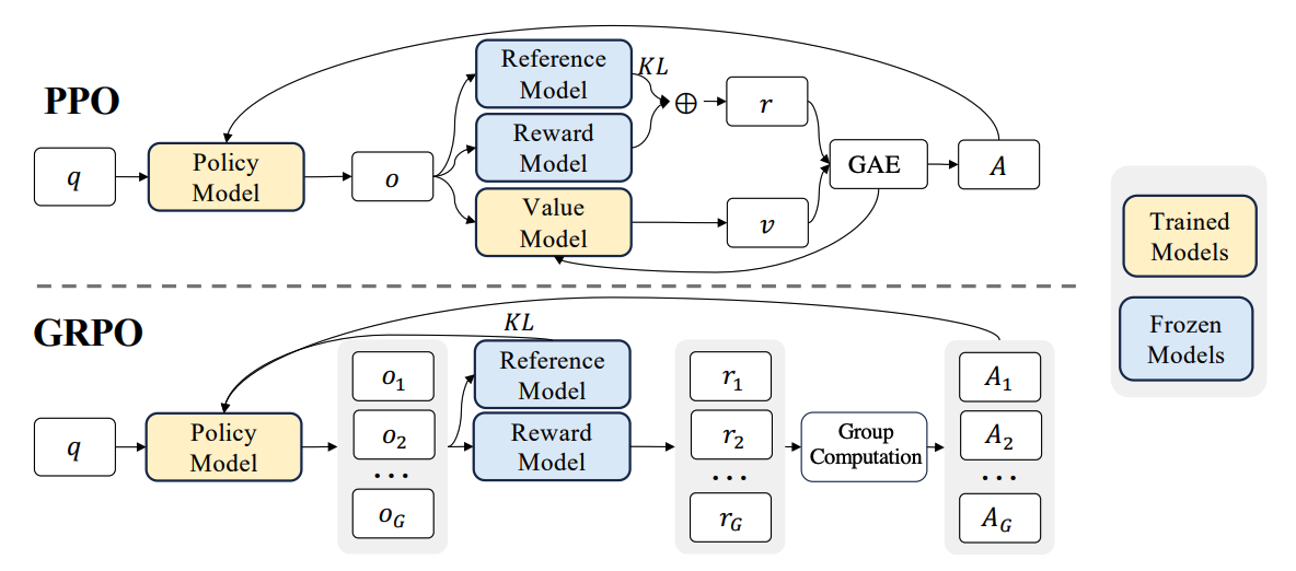
PPO is widely used in the RL fine-tuning stage of LLMs, which optimizes LLMs by maximizing the following surrogate objective (we use the form given in the DeepSeekMath paper here):
\[\begin{equation} \begin{align*} \mathcal{J}_{PPO}(\theta) = & \mathbb{E}_{q\sim P(Q),o\sim \pi_{\theta_{old}}(O\vert q)} \frac{1}{\vert o\vert}\sum_{t=1}^{\vert o\vert} \\ & \min\left[ \frac{\pi_\theta(o_t\vert q, o_{<t})}{\pi_{\theta_{old}}(o_t\vert q, o_{<t})} A_t, \mathrm{clip}\left(\frac{\pi_\theta(o_t\vert q, o_{<t})}{\pi_{\theta_{old}}(o_t\vert q, o_{<t})}, 1-\varepsilon, 1+\varepsilon\right) A_t \right], \end{align*} \end{equation}\]where $q, o$ are questions and outputs sampled from the question dataset and old policy $\pi_{\theta_{old}}$, resepectively. By the way, the squared error and the entropy terms are omitted here compared to Eq.(15).
In the standard manner of PPO, the value function needs to be trained alongside the policy model. To mitigate over-optimization of the reward model, the standard approach is to add a per-token KL penalty from a reference model in the reward at each token, i.e.,
\[\begin{equation} r_t = r_\varphi (q, o_{\leq t}) - \beta\log\frac{\pi_\theta(o_t\vert q, o_{<t})}{\pi_{ref}(o_t\vert q, o_{<t})}, \end{equation}\]where $r_\phi$ is the reward model, $\pi_{ref}$ is the reference model and $\beta$ is the coefficient of the KL penalty. Note that the KL term here means something different than the KL term in TRPO: In TRPO, the term represents the divergence between the current policy and the previous policy; but in this context, the KL term represents the divergence between the current policy and the reference policy.
As the value model and policy model are typically similar in terms of size, this leads to significant memory and computational overhead. Moreover, in RL training, the value function is used as a baseline when computing the advantage for variance reduction. However, in mathematical reasonings or code implementations, typically only the final token receives a reward signal from the reward model, which can make it more difficult to train a value function that accurately estimates rewards at every token position.
Group Relative Policy Optimization (GRPO) is proposed to address these issues. For each question $q$, GRPO samples a group of outputs ${o_1, o_2, \cdots, o_G}$ from the old policy $\pi_{\theta_{old}}$ and then optimizes the policy model by maximizing the following objective:
\[\begin{equation} \begin{align*} \mathcal{J}_{GRPO} = & \mathbb{E}_{q\sim P(Q), \{o_i\}_{i=1}^G\sim \pi_{old}(O\vert q)} \frac{1}{G}\sum_{i=1}^G \frac{1}{\vert o_i\vert}\sum_{t=1}^{\vert o_{i}\vert} \\ & \left\{ \min\left[ \frac{\pi_\theta(o_{i,t}\vert q, o_{i,<t})}{\pi_{\theta_{old}}(o_{i,t}\vert q, o_{i,<t})}\hat{A}_{i,t}, \mathrm{clip}\left( \frac{\pi_\theta(o_{i,t}\vert q, o_{i,<t})}{\pi_{\theta_{old}}(o_{i,t}\vert q, o_{i,<t})}, 1-\varepsilon, 1+\varepsilon \right) \hat{A}_{i,t} \right] -\beta\mathbb{D}_{KL}\left[ \pi_\theta\Vert\pi_{ref} \right] \right\} \end{align*} \end{equation}\]where $\varepsilon$ and $\beta$ are hyper-paramters, and $\hat{A}_{i,t}$ is the advantage calculated based on relative rewards of the outputs inside each group only.
Different from the KL penalty term used in Eq.(20), the KL divergence in Eq.(21) is estimated with the following unbiased estimator:
\[\begin{equation} \mathbb{D}_{KL}\left[\pi_\theta\Vert\pi_{ref}\right] = \frac{\pi_{ref}(o_{i,t}\vert q, o_{i, <t})}{\pi_\theta(o_{i,t}\vert q, o_{i, <t})} - \log \frac{\pi_{ref}(o_{i,t}\vert q, o_{i,<t})}{\pi_\theta(o_{i,t}\vert q, o_{i,<t})} - 1, \end{equation}\]which is guaranteed to be positive.
Code
The detailed implementation is open-sourced at github: bizzare-rl. Successfully run the experiments on a single NVIDIA H800 card with CUDA 12.4.
Most of the code comes from the following two repositories:
- verl: A Flexible and Efficient RL Post-Training Framework
- Train transformer language models with reinforcement learning.
PPO
We’ll start by implementing the advantage calculation. Consider computing advantage $A_t$ with generalized advantage estimation (GAE):
\[\begin{equation} A_t=\delta_t+(\gamma\lambda)\delta_{t+1}+\dots+(\gamma\lambda)^{T-t+1}\delta_{T-1} \quad\text{where}\quad \delta_t=r_t+\gamma V(s_{t+1})-V(s_t), \end{equation}\]we can see that the recursive formula for the advantage can be expressed as:
\[\begin{equation} A_t = \delta_t + (\gamma\lambda)A_{t+1}. \end{equation}\]Thus we can write the function as
import verl.utils.torch_functional as verl_F

def compute_gae_advantage(
    token_level_rewards: torch.Tensor,  # (B,T) Reward of every token.
    values: torch.Tensor,  # (B,T) State value from the critic model.
    response_mask: torch.Tensor,  #(B,T) [EOS] mask.
    gamma: torch.Tensor,  # Discount factor.
    lam: torch.Tensor,  # Lambda.
):
    with torch.no_grad():
        last_gae_lam = 0
        advantages_reversed = []
        gen_len = token_level_rewards.shape[-1]

        # t = T-1, T-2, ..., 0
        for t in reversed(range(gen_len)):
            next_values = values[:, t + 1] if t < gen_len - 1 else 0.0
            # delta_t = r_t + gamma * V(s_{t+1}) - V(s_t)
            delta = token_level_rewards[:, t] + gamma * next_values - values[:, t]
            # A_t = delta_t + gamma * lambda * A_{t+1}
            last_gae_lam = delta + gamma * lam * lastgaelam
            advantages_reversed.append(last_gae_lam)
        advantages = torch.stack(advantages_reversed[::-1], dim=1)  # (B,T)

        # R_t = A_t + V(s_t)
        returns = advantages + values
        # Whitening
        ## Essentially equivalent to standardization,
        ## i.e. \hat{A} = (A - mu) / (sigma + epsilon)
        # Mask
        ## In NLP, a batch is typically: [ prompt tokens | response tokens | padding ].
        ## Only response tokens are needed for policy gradient.
        ## So we only calculate the mean/std on tokens where mask=1,
        ## and normalize the advantage only at those specific positions.
        advantages = .masked_whiten(advantages, response_mask)
    return advantages, returns
Then we can move on to the whole policy loss. But before implementation, a trick that is very commonly used in practical PPO training needs to be introduced, Dual-Clip.
Consider the case where the advantage is positive. When $\frac{\pi_\theta}{\pi_{old}}$ increases, loss tends to decrease, which is exactly the optimizer wants to see. Meanwhile, we want to control this ratio to prevent it from getting too large. The clip mechanism does a great job of achieving this.
But let’s look at the case when the advantage is negative. Increasing this probability ratio now increases the loss, so the optimizer is incentivized to reduce this ratio, i.e., decrease the probability of the sampled action. This is consistent with discouraging bad actions. However, an important subtlety is that this lower clipping does not symmetrically bound the magnitude of the loss when r grows large. In the region where the ratio is greater than $1+\epsilon$, the unclipped term dominates for $A<0$ and the loss continues to grow approximately linearly with the ratio. As a result, extremely large ratios combined with negative advantages can still produce disproportionately large loss contributions. So we need an extra bound to address this instability, which leads to the introduction of dual-clip.
import verl.utils.torch_functional as verl_F

def compute_policy_loss(
    old_log_prob,  # log(π_old(a|s))
    log_prob,  # log(π_θ(a|s))
    advantages,
    response_mask,
    cliprange=None,  # ε
    cliprange_low=None,  # Specified lower bound of clip.
    cliprange_high=None,  # Specified higher bound of clip.
    clip_ratio_c=3.0,  # Lower bound ratio of dual-clip
    loss_agg_mode: str = "token-mean",
):
    assert clip_ratio_c > 1.0

    # π_θ(a|s) / π_old(a|s) = e ^ (log(π_θ(a|s)) - log(π_old(a|s)))
    negative_approx_kl = log_prob - old_log_prob
    ratio = torch.exp(negative_approx_kl)

    # E[log(π_old(a|s)) - log(π_θ(a|s))]
    ppo_kl = verl_F.masked_mean(-negative_approx_kl, response_mask)

    # CPI loss
    pg_losses1 = -advantages * ratio

    # Clip range: clip or dual-clip
    if cliprange_low is None:
        cliprange_low = cliprange
    if cliprange_high is None:
        cliprange_high = cliprange

    # Clip loss
    ## - clip(ratio, 1-cliprange, 1+cliprange) * A
    pg_losses2 = -advantages * torch.clamp(ratio, 1 - cliprange_low, 1 + cliprange_high)
    ## max(-ratio * A, -clip(ratio, 1-cliprange, 1+cliprange) * A)
    clip_pg_losses1 = torch.maximum(pg_losses1, pg_losses2)
    # Calculate the proportion of clipping occurrences.
    ## Too high: clipping is too strong and learning is being restricted;
    ## Too low: clipping is too weak.
    pg_clipfrac = verl_F.masked_mean(
        torch.gt(pg_losses2, pg_losses1).float(),
        response_mask
    )

    # Dual-Clip loss
    pg_losses3 = -advantages * clip_ratio_c
    ## min(- A * c, L_{CLIP})
    clip_pg_losses2 = torch.min(pg_losses3, clip_pg_losses1)
    ## Monitor whether negative advantage is being excessively restricted.
    pg_clipfrac_lower = verl_F.masked_mean(
        torch.gt(clip_pg_losses1, pg_losses3) * (advantages < 0).float(),
        response_mask
    )

    # Final loss
    ## Positive A: clip
    ## Negative A: dual-clip
    pg_losses = torch.where(advantages < 0, clip_pg_losses2, clip_pg_losses1)
    # Aggregate loss tensor into scalar value based on the chosen mode.
    pg_loss = agg_loss(
        loss_mat=pg_losses,
        loss_mask=response_mask,
        loss_agg_mode=loss_agg_mode
    )

    return pg_loss, pg_clipfrac, ppo_kl, pg_clipfrac_lower
Remember the squared error and the entropy terms that were omitted?
def compute_value_loss(
    values_pred: torch.Tensor,  # Predicted values.
    values: torch.Tensor,  # Baseline values.
    returns: torch.Tensor,  # Ground truth returns.
    response_mask: torch.Tensor,
    cliprange_value: float,  # Clip range for predicted values.
    loss_agg_mode: str = "token-mean"
):
    values_pred_clipped = verl_F.clip_by_value(
        values_pred,
        values - cliprange_value,
        values + cliprange_value
    )
    vf_losses1 = (values_pred - returns) ** 2
    vf_losses2 = (values_pred_clipped - returns) ** 2
    clipped_vf_losses = torch.max(vf_losses1, vf_losses2)
    vf_loss = agg_loss(
        loss_mat=clipped_vf_losses,
        loss_mask=response_mask,
        loss_agg_mode=loss_agg_mode
    )
    vf_clipfrac = verl_F.masked_mean(
        torch.gt(vf_losses2, vf_losses1).float(),
        response_mask
    )
    return vf_loss, vf_clipfrac

def compute_entropy_loss(
    logits,
    response_mask,
    loss_agg_mode: str = "token-mean"
):
    # compute entropy
    token_entropy = verl_F.entropy_from_logits(logits)  # (bs, response_len)
    entropy_loss = agg_loss(
        loss_mat=token_entropy,
        loss_mask=response_mask,
        loss_agg_mode=loss_agg_mode
    )
    return entropy_loss
Once all these key components are complete, we can look into building the trainer for PPO.
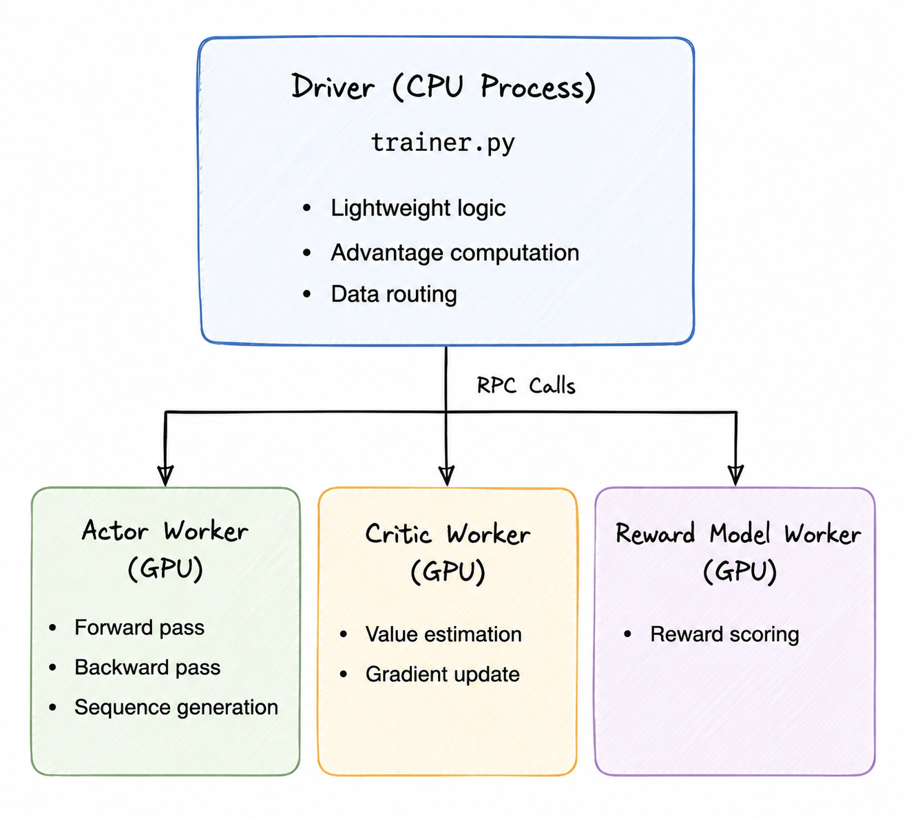
All the engineering, distributed, asynchronous, logging, verification, and complex analysis components have been removed, and the following code only shows the core logic.
class PPOTrainer:
    def __init__(self, config, ...):
        """Constructor of the trainer."""

        self.config = config
        # ... (omitted)

    def _load_checkpoint(self):
        # ... (omitted)

    def init_workers(self):
        self.actor = ...
        self.critic = ...
        self.ref_policy = ...
        self.reward_model = ...
        # ... (omitted)

    def fit(self):
        """Minimal training loop."""

        self.global_steps = 0

        # Load checkpoint.
        self._load_checkpoint()

        for epoch in range(self.config.trainer.total_epochs):
            for batch_dict in self.train_dataloader:
                # DataProto
                ## A data structure that aims to provide a standard protocol for data exchange between functions.
                ## Contains a batch (TensorDict) and a meta_info (Dict).
                # TensorDict
                ## Allows you to manipulate a dictionary of Tensors like a single Tensor.
                ## https://docs.pytorch.org/tensordict/stable/index.html
                batch = DataProto.from_single_dict(batch_dict)

                # ===== rollout =====
                gen_inputs = batch.pop(
                    batch_keys=["input_ids", "attention_mask", "position_ids"],
                    non_tensor_batch_keys=["raw_prompt_ids"],
                )
                rollout_output = self.actor.generate_rollout_sequences(gen_inputs)
                batch = batch.union(rollout_output)

                batch.batch["response_mask"] = compute_response_mask(batch)

                # ===== reward =====
                reward_tensor = self.reward_model.compute_rm_score(batch)
                batch = batch.union(reward_tensor)

                reward_tensor = compute_reward(batch, self.reward_fn)
                batch.batch["token_level_rewards"] = reward_tensor

                # ===== reference policy KL penalty =====
                ref_log_prob = self.ref_policy.compute_ref_log_prob(batch)
                batch = batch.union(ref_log_prob)
                batch = apply_kl_penalty(batch, kl_ctrl=self.kl_ctrl_in_reward)

                # ===== critic value =====
                values = self.critic.compute_values(batch)
                batch = batch.union(values)

                # ===== advantage estimation =====
                batch = compute_advantage(
                    batch,
                    adv_estimator=self.config.algorithm.adv_estimator,
                    gamma=self.config.algorithm.gamma,
                    lam=self.config.algorithm.lam,
                )

                # ===== critic update =====
                critic_out = self.critic.update_critic(batch)

                # ===== actor update =====
                actor_out = self.actor.update_actor(batch)

                # ===== end of the loop =====
                self.global_steps += 1
                if self.global_steps >= self.total_training_steps:
                    return
GRPO
We can implement the advantage calculation as follow.
def compute_grpo_outcome_advantage(
    token_level_rewards: torch.Tensor,
    response_mask: torch.Tensor,
    index: np.ndarray,  # Group ID per sample
    epsilon: float = 1e-6,
):
    """Compute advantage for GRPO, operating only on outcome scalar reward."""

    # Compute total reward for each response.
    scores = token_level_rewards.sum(dim=-1)  # (B,T) -> (B,)

    id2score = defaultdict(list)
    id2mean = {}
    id2std = {}

    with torch.no_grad():
        # Group by index.
        bsz = scores.shape[0]
        for i in range(bsz):
            id2score[index[i]].append(scores[i])

        # Compute mean and std for each group.
        for idx in id2score:
            if len(id2score[idx]) == 1:
                id2mean[idx] = torch.tensor(0.0)
                id2std[idx] = torch.tensor(1.0)
            elif len(id2score[idx]) > 1:
                id2mean[idx] = torch.mean(torch.tensor(id2score[idx]))
                id2std[idx] = torch.std(torch.tensor([id2score[idx]]))
            else:
                raise ValueError(f"no score in prompt index: {idx}")

        # Compute advantage for each response.
        for i in range(bsz):
            scores[i] = (scores[i] - id2mean[index[i]]) / (id2std[index[i]] + epsilon)

        # Broadcast scalar advantage to token-level.
        scores = scores.unsqueeze(-1) * response_mask  # (B,) -> (B,T)

    # Return identical advantages and returns.
    return scores, scores
The implementation of computing policy loss is exactly the same with PPO, so let’s directly jump into the training loop.
class GRPOTrainer(PPOTrainer):
    def __init__(self, config, ...):
        """Constructor of the trainer."""

        self.config = config
        # ... (omitted)

    def fit(self):
        """Minimal training loop."""

        self.global_steps = 0

        # Load checkpoint.
        self._load_checkpoint()

        for epoch in range(self.config.trainer.total_epochs):
            for batch_dict in self.train_dataloader:
                if self.global_steps >= self.total_training_steps:
                    return

                # ===== build prompt batch =====
                batch = DataProto.from_single_dict(batch_dict)

                gen_inputs = batch.pop(
                    batch_keys=["input_ids", "attention_mask", "position_ids"],
                    non_tensor_batch_keys=["raw_prompt_ids"],
                )

                # ===== rollout: generate responses =====
                gen_output = self.actor.generate_rollout_sequences(gen_batch)

                # Generate multiple responses for each prompt.
                batch.non_tensor_batch["uid"] = np.array(
                    [str(uuid.uuid4()) for _ in range(len(batch.batch))],
                    dtype=object,
                )
                batch = batch.repeat(
                    repeat_times=self.config.actor_rollout_ref.rollout.n,
                    interleave=True,
                )
                batch = batch.union(gen_output)

                batch.batch["response_mask"] = compute_response_mask(batch)

                # ===== compute reward =====
                reward_tensor, reward_extra_infos = compute_reward(
                    batch,
                    self.reward_fn,
                )

                batch.batch["token_level_scores"] = reward_tensor

                # Add token-level KL penalty.
                batch, _ = apply_kl_penalty(
                    batch,
                    kl_ctrl=self.kl_ctrl_in_reward,
                    kl_penalty=self.config.algorithm.kl_penalty,
                )

                # ===== compute old policy log probs =====
                old_log_prob = self.actor.compute_log_prob(batch)
                old_log_prob.batch.pop("entropys", None)
                batch = batch.union(old_log_prob)

                # ===== compute reference policy log probability =====
                ref_log_prob = self.ref_policy.compute_ref_log_prob(batch)
                batch = batch.union(ref_log_prob)

                # ===== compute advantage =====
                batch = compute_advantage(
                    batch,
                    adv_estimator=self.config.algorithm.adv_estimator,
                    gamma=self.config.algorithm.gamma,
                    lam=self.config.algorithm.lam,
                    num_repeat=self.config.actor_rollout_ref.rollout.n,
                )

                # ===== update actor =====
                if self.global_steps >= self.config.trainer.critic_warmup:
                    batch.meta_info["multi_turn"] = (
                        self.config.actor_rollout_ref.rollout.multi_turn.enable
                    )
                    self.actor.update_actor(batch)

                self.global_steps += 1
References
[1] John Schulman, Filip Wolski, Prafulla Dhariwal, Alec Radford, Oleg Klimov. (2017). Proximal Policy Optimization Algorithms.
[2] Zhihong Shao, Peiyi Wang, Qihao Zhu, Runxin Xu, Junxiao Song, Mingchuan Zhang, Y.K. Li, Y. Wu, Daya Guo. (2024). DeepSeekMath: Pushing the Limits of Mathematical Reasoning in Open Language Models.