Evolutionary AI System for Scientific Discovery
This blog is basically a review of FunSearch and AlphaEvolve.
Suppose we had an AI system capable of formulating scientific hypotheses, reading the literature, writing simulation code, designing experiments, and analyzing results. Then we can simply input a research problem or hypothesis, hoping it will provide a one-shot solution or answer.
But would merely doing that be sufficient to produce genuinely novel scientific discoveries?
The problem is that scientific discovery rarely emerges from a single “generation”. It typically involves an iterative cycle:
- propose candidates (solutions, hypothesis, …)
- evaluate and test
- identify problems
- revise
- test again
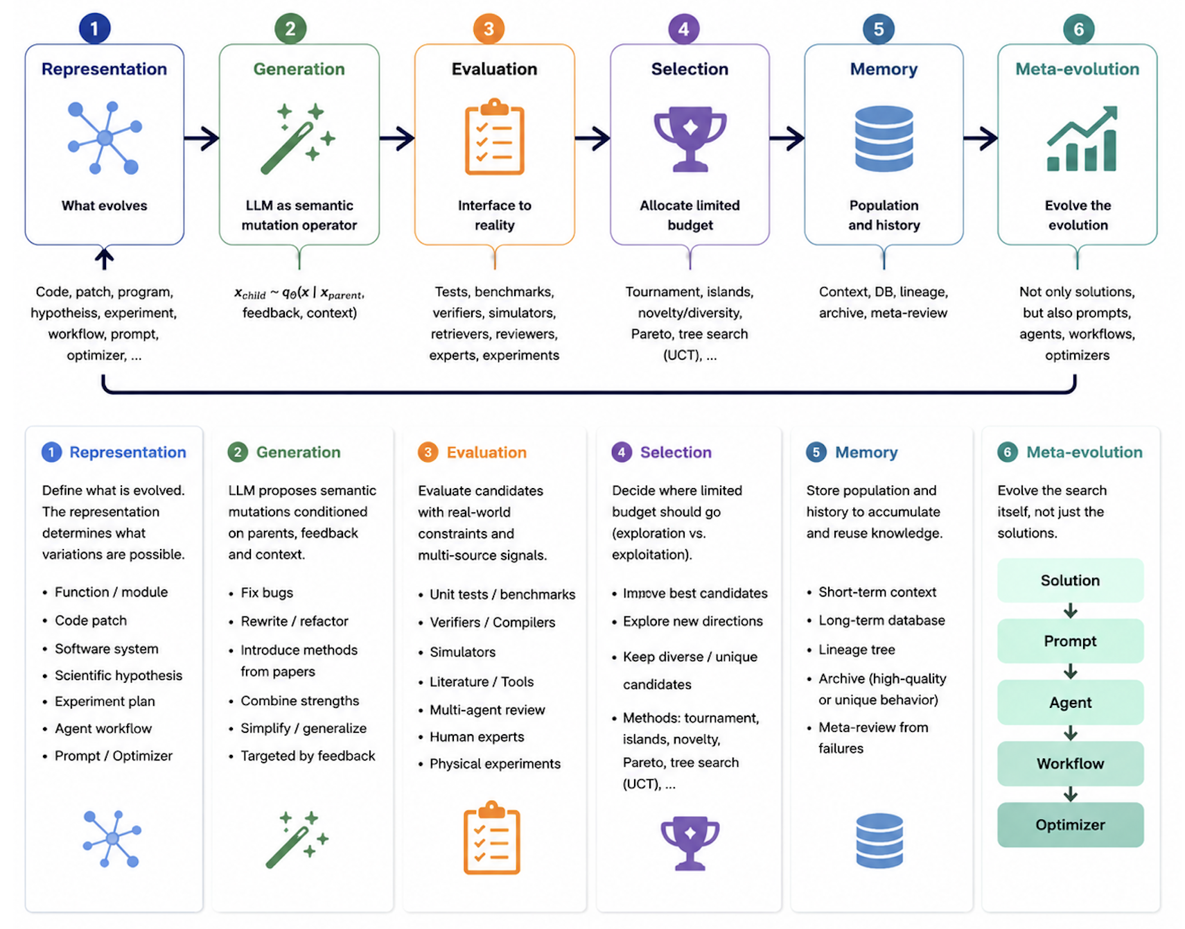
This has the same basic structure as evolutionary search. So it’s believed that AI for scientific discovery is not about having a more powerful model directly produce answers; rather, it is about organizing LLMs or LLM-based agents, tools, evaluators, external memory, and resource scheduling into a system capable of conducting long-horizon search, accumulating knowledge, and continuously improving itself.
From Optimization to Search
Richard Sutton: “One thing that should be learned from the bitter lesson is the great power of general purpose methods, of methods that continue to scale with increased computation even as the available computation becomes very great. The two methods that seem to scale arbitrarily in this way are search and learning.”
Assume finding the solution to a scientific problem can be modeled as:
\[\begin{equation} x^*=\underset{x\in\mathcal{X}}{\operatorname{argmax}}\,R(x), \end{equation}\]where $\mathcal{X}$ represents the set of all candidate solutions, and $R(x)$ is the evaluation function used to measure the quality of the solution.
From an optimization perspective, this is a search problem: we aim to find a program that maximizes the evaluation function within a vast search space $\mathcal{X}$. However, unlike neural network parameter optimization, the solution space is typically discrete and structurally complex. Take programs for example, modifying a program does not correspond to a small movement in a continuous space:
From
def heuristic(x):
    return x.size
to
def heuristic(x):
    return x.size ** 2
though the code change is minimal, the resulting behavior may change significantly. Therefore, program spaces generally do not possess exploitable continuous structures, and the search process cannot be directly guided by local information such as gradients.
However, for any candidate program, we can typically:
- Generate the program;
- Execute the program;
- Determine whether it satisfies the constraints;
- Compute its performance score based on task-specific metrics.
This type of property is usually summarized as hard to solve but easy to evaluate.
A natural approach to this kind of search problem is to continuously generate new candidate programs, use the evaluation function to select better candidates, and repeat this process. For example, suppose a machine has chosen an number between 1 and 100. We first make an arbitrary guess (generate) and receive feedback indicating whether the guess is too high or too low (evaluate). Based on this feedback, we iteratively narrow the search range and make new guesses until we identify the correct number.
Evolutionary Search
Here I want to introduce evolutionary search, since it’s the fundemental idea behind the evolutionary components following. Code is implemented in Google Colab.
Evolutionary search is a population-based stochastic search method that maintains a set of candidate solutions and continuously generates better candidate solutions through mutation, recombination, evaluation, and selection.
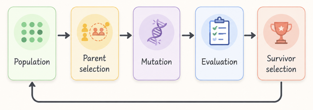
Let the population at generation $t$ be:
\[P_t=\{x_t^{(1)}, x_t^{(2)}, \dots, x_t^{(N)}\}\]where each candidate $x_t^{(i)}$ is called an individual in the population.
Step 1: Select several individuals from the current population that are worth further exploration:
\[\begin{equation} x_\text{parent}\sim \mathrm{Select}(P_t,R) \end{equation}\]For multiple individuals in a population, if we want to use an algorithm to obtain the best candidates, we need a metric to evaluate the quality of each individual. We call this metric fitness, which corresponds to the evaluation function $R$ in the example above.
A common selection strategy is tournament selection. Specifically, we randomly sample $k$ individuals from the population and choose the best individual with probability $p$, the second best with probability $p(1-p)$, the third best with probability $p((1-p)^2)$, so on.
Then we just call this strategy multiple times to gain the parent individuals. The reason we cannot simply select only a single individual is due to the exploration–exploitation trade-off:
- Exploitation: If the selection pressure is too strong, and we only select the best individuals for reproduction, the entire search process degenerates into a single greedy trajectory. Although this leads to faster convergence, population diversity quickly disappears, making the search prone to getting trapped in local optima.
- Exploration: If the selection pressure is too weak, we maintain rich population diversity, but a large amount of computational budget is spent evaluating low-quality candidates. As a result, performance improvement becomes slow.
Step 2: Mutation. We usually refer to the program itself as genotype, while the behavior or output produced by executing the program is called phenotype. Mutation introduces perturbations to the genotype of the candidate obtained from the previous step:
\[\begin{equation} x_\text{child}=M(x_\text{parent}) \end{equation}\]For example, in LLM-based program search, this step may involve modifying expressions in an algorithm, rewriting the logic of key functions, fixing bugs, or making other program-level changes.
When generating offspring from a parent, we sometimes want to combine the strengths of multiple candidate individuals. The process of combining information from multiple parents to produce offspring is called crossover. In LLM-based program search, this can be implemented by placing two candidate programs into the context and allowing the LLM to compare them and incorporate desirable components from both.
Step 3: Evaluate the mutated candidate:
\[\begin{equation} s_\text{child}=R(x_\text{child}) \end{equation}\]Here, the object being evaluated is the phenotype of the offspring.
Step 4: Select survivors from the parents and offspring to form the next generation:
\[\begin{equation} P_{t+1}=\mathrm{Survive}(P_t\cup C_t,f) \end{equation}\]Here, we allow two generations of populations to compete with each other, ensuring that the best candidate individuals are not lost. This mechanism is known as elitism.
General Framework
A general framework of the system can be formed as the following picture shows:
FunSearch
In FunSearch, the search target is a function $f$, which generates solutions through the function:
\[\begin{equation} x=f(z) \end{equation}\]where $z$ is the problem input. Therefore, the optimization objective (Eq. (1)) becomes:
\[\begin{equation} f^*=\underset{f\in\mathcal{P}}{\operatorname{argmax}}\, R(f) \end{equation}\]where $\mathcal{P}$ is the program space.
FunSearch typically does not allow the agent to modify the entire software system. Instead, it only modifies a key function within the system. Let the entire solving program be denoted as $S[f]$, where $S$ is a fixed program framework (also called the skeleton); $f$ is the key function that FunSearch is allowed to modify; and $S[f]$ represents the complete program obtained by inserting function $f$ into the skeleton $S$.
In programming, we usually use a set of test cases to determine whether a program is functionally correct. Let the evaluation set be:
\[D=\{z_1,z_2,\dots,z_r\}\]where each $z_i$ is an evaluation input. For a candidate function $f$, the complete program receives a score on input $z_i$:
\[\begin{equation} e_i(f)=E(S[f],z_i) \end{equation}\]where $E$ is the evaluator, and $e_i(f)$ is the score of function $f$ on the $i$-th input. The scores of the candidate program across different inputs are combined through an aggregate function $A$ as:
\[\begin{equation} J(f)=A(e_1(f),e_2(f),\dots,e_r(f)) \end{equation}\]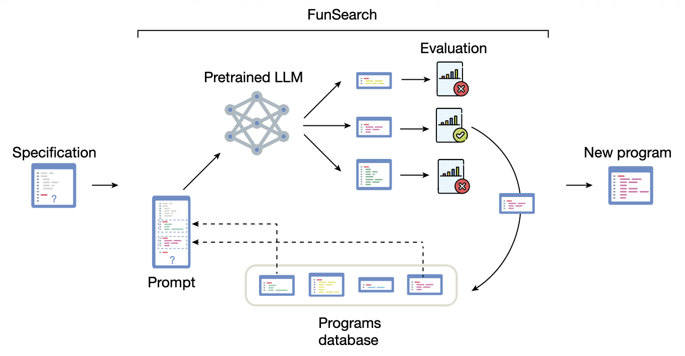
Specification
The Specification provides a complete definition of the modifiable function interface, the fixed program skeleton, the evaluation methodology, and the tools available to the system. It includes:
- The name of the modifiable function;
- The input and output types;
- A description of the function;
- The fixed solving framework;
- The evaluator;
- The initial function implementation;
- The libraries or auxiliary functions that can be used.
Evaluator
The Evaluator is responsible for assessing candidate programs from three perspectives:
- Syntactic validity: whether the code can be successfully parsed by the compiler.
- Execution validity: whether the program terminates within the specified time limit, stays within the memory constraints, and does not raise runtime exceptions.
- Output validity and quality: whether the output satisfies the problem constraints and what quality score the output achieves.
Program Database
The Program Database is a persistent storage component that maintains valid candidate programs, their scores on different inputs, their aggregated performance scores, and the populations they belong to. It serves as an external memory system: information stored outside the model parameters that can be accessed and updated by the search process.
Islands
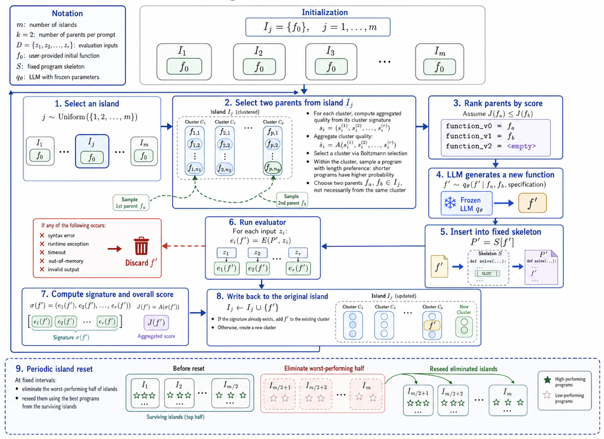
In details, the database is viewed as a population, divided into multiple relatively independent subpopulations (islands). Assume that $m$ islands are initialized:
\[I_1,I_2,...,I_m.\]Given the initial program $f_0$, each island starts from the same program:
\[\begin{equation} I_j=\{f_0\},\quad j=1,\dots,m. \end{equation}\]After initialization, each island independently evolves its own subpopulation.
Whenever a prompt needs to be constructed:
- Select an island $I_j$ uniformly at random;
- Select parent programs only from this island;
- Generate a new program from the selected parents;
- After evaluation, store the new program back into the same island.
Every certain period of time, the best program from each island is compared:
\[\begin{equation} B_j=\max_{f\in I_j}J(f) \end{equation}\]The replacement process is then performed as follows:
- Identify the bottom half of islands according to their best program scores;
- Clear these islands;
- For each cleared island, randomly select a surviving island;
- Copy the best program from the surviving island into the cleared island;
- Restart the search process from this copied program.
Signature Clustering
An island can be further divided into several clusters. A cluster is a group of objects that are considered similar according to a given similarity criterion. In FunSearch, programs with identical signatures are assigned to the same cluster.
The signature of a candidate program $f$ is a vector consisting of its individual scores across $r$ evaluation inputs:
\[\sigma(f) = (e_1(f),e_2(f),\dots,e_r(f))\]After selecting an island as said earlier, FunSearch first samples a cluster and then samples a program from within that cluster. Let the signature of cluster $C_i$ be:
\[s_i=(s_{i}^{(1)},s_i^{(2)},\dots,s_i^{(r)})\]FunSearch applies Boltzmann Selection to determine the probability of selecting each cluster:
\[\begin{equation} P(C_i)=\frac{\exp(\bar{s}_i/T)}{\sum_{j}\exp(\bar{s}_j/T)} \end{equation}\]where $\bar{s}i=A(s{i}^{(1)},s_i^{(2)},\dots,s_i^{(r)})$ represents the aggregated quality of cluster $C_i$; $T$ is the temperature parameter, which controls the concentration of the probability distribution: A larger $T$ produces a probability distribution closer to uniform sampling (exploration), while a smaller $T$ concentrates the probability mass on high-performing candidates (exploitation).
The temperature can be periodically adjusted according to the number of programs in an island:
\[\begin{equation} T_\text{cluster}=T_0\left(1-\frac{n\,\mathrm{mod}\,N}{N}\right) \end{equation}\]where: $n$ is the current number of programs in the island; $N$ is the predefined cycle length; $T_0$ is the initial temperature.
After selecting a cluster, FunSearch favors sampling shorter programs. Let the length of a program be $L(f)$, measured by the number of characters. The preference can be conceptualized as:
\[\begin{equation} P(f\vert C_i) \propto \exp\left(-\frac{\tilde{L}(f)}{T_\text{program}}\right) \end{equation}\]where $\tilde{L}(f)$ is the normalized program length; $T_\text{program}$ is the temperature parameter controlling the preference for shorter programs.
Prompt Builder
FunSearch does not simply provide the LLM with the single “current best program.” Instead, it selects multiple programs from the database and constructs a prompt that presents them in an ordered sequence of improvements. This approach is known as best-shot prompting, where the model is guided by a set of progressively improved examples rather than a single solution.
Best-shot prompting selects high-scoring programs from historical candidates, arranges these programs in ascending order according to their scores, and instructs the LLM to generate the next improved version.
Assume that the selected two programs satisfy:
\[\begin{equation} J(f_a)<J(f_b) \end{equation}\]The constructed prompt can be represented as:
def priority_v0(x):
    # lower score implementation
    ...

def priority_v1(x):
    # higher score implementation
    ...

def priority_v2(x):
    # TODO
If only a single best-performing program is provided, the LLM receives just a static point $f_{\text{best}}$. However, if two programs with different performance levels are provided, the LLM can also infer an implicit improvement trajectory:
\[\begin{equation} f_\text{low}\rightarrow f_\text{high} \end{equation}\]This provides the LLM with semantic information about a possible direction for further improvement.
Pipeline
Thus the detailed pipeline of FunSearch is shown in the following picture.
AlphaEvolve
AlphaEvolve can be viewed as a large-scale and generalized extension of FunSearch.
| FunSearch | AlphaEvolve |
|---|---|
| Modify a key function | Modify multiple code blocks |
| Single score | Multi-metric evaluation |
| Complete function generation | Structured code patching |
| Fixed prompts | Rich history, feedback, and domain context |
| Single-layer evaluation | Evaluation cascade |
AlphaEvolve targets problems with machine-gradeable solution, which can be automatically evaluated by computer programs and assigned one or more quantitative metrics. Given a candidate program $P$, the evaluation function can be represented as:
\[E(P)=(m_1(P),m_2(P),\dots,m_d(P))\]where $E$ is the evaluation function, $m_i(P)$ represents the $i$-th evaluation metric, and $d$ is the number of metrics.
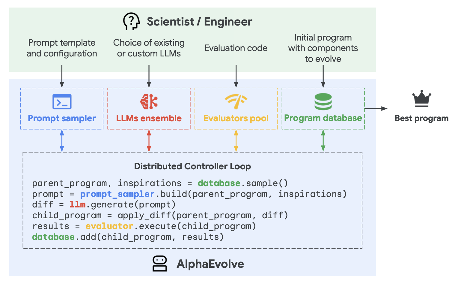
The overall architecture of AlphaEvolve can be summarized as integration of the following components:
- Task Specification: defines which parts of the code can evolve and how candidates are evaluated;
- Prompt Sampler: constructs prompts from historical programs and contextual information;
- LLM Ensemble: generates candidate code modifications;
- Patch Applier: applies modifications to the existing code through patches;
- Evaluators: execute and rate candidate programs;
- Evolutionary Database: stores results and selects future parent candidates.
Task Specification
Evaluation Function
AlphaEvolve requires users to provide an evaluation function that maps candidate programs to measurable metrics:
def evaluate(eval_inputs) -> dict[str, float]:
    ...
    return metrics
The returned metrics define the performance of each candidate and determine whether it should survive in the evolutionary process.
Evolution Blocks
AlphaEvolve allows users to explicitly specify modifiable regions using special markers:
# EVOLVE-BLOCK-START

def optimizer():
    ...

def loss_function():
    ...

# EVOLVE-BLOCK-END
The remaining code stays unchanged and serves as the fixed program skeleton.
Compared with FunSearch, which usually evolves only a single function, AlphaEvolve supports multiple evolution blocks. These blocks can contain classes, functions, configurations, or even complete algorithmic components.
Prompt Sampling
The prompts used by AlphaEvolve contain substantially more information than those in FunSearch. A typical prompt can be expressed as:
\[p=\mathrm{Compose}(\text{instructions},\text{context},\text{prior programs},\text{current program},\text{evaluation feedback})\]where $\mathrm{Compose}$ represents the process of combining multiple information sources into a single input for the LLM.
Prior programs are previously generated candidates stored in the evolutionary database. Similar to FunSearch’s best-shot prompting, AlphaEvolve uses historical candidates as examples to guide future generations. However, AlphaEvolve can provide much richer information, including:
- multiple previous programs;
- complete code implementations;
- multiple evaluation metrics for each candidate;
- execution outputs;
- natural-language feedback;
- domain-specific knowledge.
Explicit context refers to additional information provided by users and directly inserted into the prompt. It may include:
- problem definitions;
- mathematical formulations;
- code snippets;
- engineering constraints;
- related research papers;
- API documentation;
- known failed approaches;
- hardware specifications.
This allows the LLM to reason not only from previous solutions but also from external domain knowledge.
Patch-Based Evolution
A key difference between FunSearch and AlphaEvolve is the way code modifications are represented.
For a small function, rewriting the entire function is often acceptable. However, when evolving a codebase containing hundreds or thousands of lines, asking an LLM to rewrite the entire file introduces several issues:
- Correct existing code may be accidentally deleted;
- Unrelated modifications may be introduced;
- Token consumption becomes significantly higher;
- It becomes difficult to determine which change caused performance improvement;
- Repeated iterations may lead to code drift, where the program gradually deviates from its original structure and accumulates unnecessary or inconsistent changes.
To solve this problem, AlphaEvolve typically requires the LLM to output a diff, which specifies exactly which existing code should be replaced and what new code should be inserted.
A patch has a structure similar to:
<<<<<<< SEARCH
return optax.adam(learning_rate)
=======
return optax.adamw(
    learning_rate,
    weight_decay=1e-4,
)
>>>>>>> REPLACE
where:
- The
SEARCHsection must exactly match the corresponding code in the current program; - The
REPLACEsection contains the new implementation.
Patch-based evolution enables precise, localized modifications while preserving the overall software structure.
LLM Ensemble
Instead of relying on a single language model, AlphaEvolve can combine multiple models or model configurations to generate candidate solutions.
For example, using Gemini 2.0 Flash and Gemini 2.0 Pro, the overall generation distribution can be represented as:
\[\begin{equation} q(P^\prime)=\lambda q_\text{Flash}(P^\prime)+(1-\lambda)q_\text{Pro}(P^\prime) \end{equation}\]where:
- $q_\text{Flash}$ and $q_\text{Pro}$ represent the candidate distributions generated by the two models;
- $\lambda\in[0,1]$ controls their relative contribution.
The ensemble approach allows different models to contribute different exploration behaviors and improves the diversity of generated candidates.
Evaluation Cascade
Large-scale code evolution requires efficient evaluation. Running expensive evaluations on every generated program would quickly become computationally infeasible.
AlphaEvolve therefore introduces an evaluation cascade, where candidates pass through multiple evaluation stages with gradually increasing costs.
A typical evaluation pipeline may contain:
Stage 0: Syntax and import checking
Stage 1: Small-scale input testing
Stage 2: Limited random seeds
Stage 3: Full evaluation dataset
Stage 4: Large-scale parallel experiments
Stage 5: Strict correctness verification
Formally, assume the cascade contains $K$ evaluation stages:
\[E_1,E_2,\dots,E_K\]with increasing costs:
\[\begin{equation} c_1<c_2<\cdots<c_K \end{equation}\]Each stage has a passing threshold $\tau_k$. A candidate program $P$ proceeds to the next stage only if:
\[\begin{equation} E_k(P)\geq\tau_k \end{equation}\]This design filters out low-quality candidates early and reserves expensive computation for promising solutions.
Meta-Prompt Evolution
A further extension of AlphaEvolve is the evolution of the prompts themselves.
A meta-prompt is a prompt designed to generate, modify, or select other prompts. Rather than evolving only candidate programs, AlphaEvolve can also evolve the strategies used to guide program generation:
- The LLM can propose new instructions and contextual information through additional prompt-generation steps;
- These meta-prompts are stored in an independent database;
- Meta-prompts can evolve together with candidate programs.
This process can be represented using two archives:
\[\begin{align*} \mathcal{A}_P &= \{\text{candidate programs}\}\\ \mathcal{A}_M &= \{\text{candidate meta-prompts}\} \end{align*}\]The search process therefore evolves both the solutions and the mechanisms used to discover solutions.
Pipeline
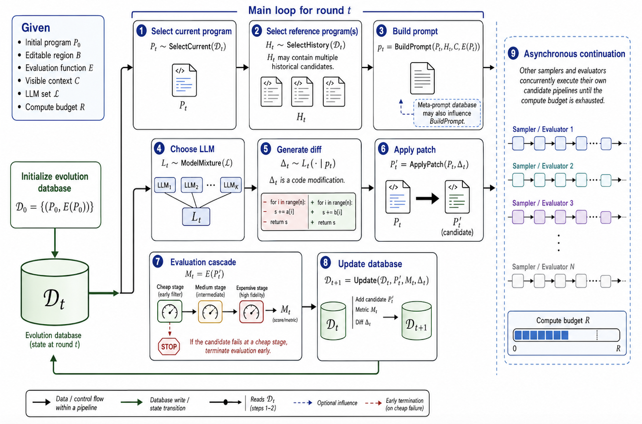
The detailed pipeline of AlphaEvolve is shown in the following picture.
Escher-Loop
While AlphaEvolve allow LLM to continuously modify its task code, the aforementioned optimization rules remain largely fixed. This leads to a potential bottleneck: if the true limiting factor for search performance is the “search method” rather than the current candidate programs, simply continuing to modify candidate programs may not be enough to overcome the plateau.
As proposed in the paper: “The core of intelligence lies not in the static mastery of a task, but in the dynamic ability to optimize both the task solution and the optimizer itself.”
Not finished.
Reference
[1] Romera-Paredes, B., Barekatain, M., Novikov, A. et al. Mathematical discoveries from program search with large language models. Nature 625, 468–475 (2024). https://doi.org/10.1038/s41586-023-06924-6
[2] Novikov, A., Vu, N., Eisenberger, M. et al. AlphaEvolve: A coding agent for scientific and algorithmic discovery. arXiv:2506.13131. https://doi.org/10.48550/arXiv.2506.13131
[3] Liu, Z., Guo, X., Wei, X. et al. Escher-Loop: Mutual Evolution by Closed-Loop Self-Referential Optimization. arXiv:2604.23472. https://doi.org/10.48550/arXiv.2604.23472