Linda S. Gottfredson: “Intelligence is a very general mental capability that, among other things, involves the ability to reason, plan, solve problems, think abstractly, comprehend complex ideas, learn quickly and learn from experience. It is not merely book learning, a narrow academic skill, or test-taking smarts. Rather, it reflects a broader and deeper capability for comprehending our surroundings—”catching on,” “making sense” of things, or “figuring out” what to do.”

In the area of modern machine learning, the term “world model” is becoming an increasingly popular, yet increasingly vague, term. It’s easy to get the intuition that a so-called world model is simply a model that can generate a realistic world, if we start from generative models nowadays. However, I think a more interesting and fundamental point about the world model is, can an intelligent agent think through its own internal world before actually taking action?

For example, if a person needs to walk from the table, which is on the left, to the door, his (or her) behavior would definitely not be: take a step to the left \(\rightarrow\) bump into the table \(\rightarrow\) receive a negative reward \(\rightarrow\) update the policy. Instead, he (or she) will first roughly judge in his (or her) mind: the table is there, and I should be able to reach the door by going around to the right. Humans do this kind of simple planning every day. Before we actually take action, we have already “run” the future in a sense.

If machines were to acquire similar capabilities, they would likely need to internally build a model of how the world works, which is precisely the starting point of the research path of world models.

This blog is basically a review of three works on this topic:

• Integrated Architectures for Learning, Planning, and Reacting Based on Approximating Dynamic Programming by Richard S. Sutton
• World Models by David Ha and Jurgen Schmidhuber
• A Path Towards Autonomous Machine Intelligence by Yann LeCun

Why do machines need to imagine?

Just like we’ve talked, an agent should deduce its best action based on its goal and some internal model capable of simulating how the world works. We call this kind of mechanism planning.

In the reinforcement learning literature, an agent decides what to do based on a certain policy, which is essentially a probability distribution of possible actions conditioned on the agent’s current state. And this policy is learned via trial-and-error in a real world, i.e., the agent learns from experiences that each actually happens once at least. We call this kind of mechanism learning.

Sometimes, we are able to perform instinctive behaviours when we face danger, or act reflectively when consolidating a specific task in repitition, without the need to consciously plan out a course of action. We call this kind of mechanism reacting.

Dyna is a class of architectures integrating and permitting tradeoffs among these three approaches, including Dyna-PI and Dyna-Q. This blog mainly introduces the latter one.

Dyna-PI

Dyna-PI is based on approximating policy iteration, which we have fully discussed in the temporal-difference learning blog. Recall that policy iteration is one of the ways of finding an optimal policy through a sequence:

where \(\xrightarrow{E}\) denotes a policy evaluation and \(\xrightarrow{I}\) denotes a policy improvement.

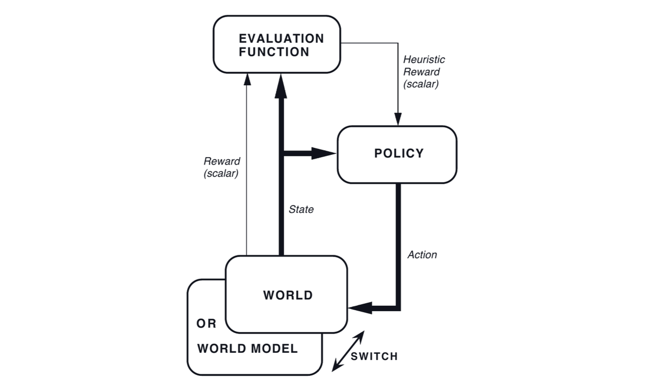
The detailed algorithm of Dyna-PI:

Now let’s deduce how Dyna-PI originates from policy iteration. To avoid confusion, we will uniformly adopt a finite discount Markov decision process (MDP):

Recall that the Bellman expectation operator is defined as:

Like we’ve talked about, policy evaluation can be seen as repeatedly applying Bellman expectation operator to the estimated state-value until convergence. And policy improvement is simply choosing a greedy action with respect to estimated state-value for each state. Policy improvement theorem gaurantees that accurate evaluation and greedy improvement will eventually lead to an optimal policy.

However, this process imposes two strict requirements on online agents:

• They must sum over all successor states;
• They must know the complete environment model.

Dyna-PI can be understood as the result of successively relaxing these three requirements.

Assume the state at current time \(t\) is \(S_t=s\). We denote the action sampled from the policy as \(A_t\sim \pi(\cdot\vert s)\). By performing the action, we can get a feedback from the world as \((S_{t+1},R_{t+1}) \sim p(\cdot, \cdot \vert s,A_t)\). The TD-error is then defined as:

We can calculate the expectation of it conditioned on the current state:

Thus the update

is a single-sample stochastic approximation of

It does not require explicitly enumerating all actions and successor states, and only require one transition sample.

In particular if \(V=v_\pi\), the expectation of TD-error conditioned on the current state and a certain action can be written as:

where \(A_\pi\) is called the advantage function, indicating how much better is the action \(a\) chosen in state \(s\) than the average performance of the current policy. Thus TD-error is also a single-sample approximation of the advantage function.

Assume the policy uses a Boltzmann distribution:

where \(w(s,a)\) is a preference parameter for every state-action pair. We can form the policy update as:

If an action produces a better action-value than the current estimated state-value (i.e., \(\delta>0\)), the preference for that action will increase; if \(\delta<0\), the preference will then decrease.

At this point, we have derived a model-free incremental algorithm from the precise policy iteration:

So where is the world model? Reinforcement learning gets real experiences from the real world, and the world model is expected to provide experiences close to reality, thus reduce the cost spended on agent-world iteractions.

Formally, we can update the world model \(\widehat{\mathcal{W}}\) with real experiences like \((s,a,s^\prime,r)\). Then we can use the model to generate a one-step hypothetical experience

Updates generated from real experience correspond to “learning”; updates generated from hypothetical experience correspond to “planning”. For each experience with the real world, \(k\) hypothetical experiences were generated with the model, representing additional planning. The larger \(k\) is, the more real-world interactions is usually saved, but more dependent it becomes on the simulation quality of the world.

Now we’ve successfully constructed a mechanism in which an agent can internally test actions and obtain corresponding possible consequences before actually taking any action.

Mr. Sutton unveiled two potential problems when Dyna-PI is applied in a changing world. One is named blocking problem, referring to the fact that the update of the systems’s behavior and the world model is too slow when adding a new barrier blocking the original optimal path; The other is named shortcut problem, referring to the fact that the system is unable to take the shortcut when removing a barrier that permitts a shorter path than the original optimal path. Dyna-Q, which is based on Q-learning, was introduced in the original paper to tackle these problems.

Where should machines imagine?

In the grid-like maze navigation task, we can simply use sequence numbers to represent states, which indicates the agent’s position in the maze. But let’s consider the case that a robot doing housework in the kitchen, which is essentially acting in the real world. The robots sees images, hears sounds, feels touch, and experiences motion continuously. So if an agent is facing an actual “real world”, what should it consider as a “state”?

Asking an agent to understand every single pixel becomes incredibly difficult, as an image contains a wealth of information: color, lighting, texture, shadows, background, entity positions, and relationships between entities. But what truly determines the agent’s next action may only be a small fraction of this information. Thus, a natural idea emerged: instead of making predictions directly in the original world, we can first compress the states of world into latent representations, i.e., encode \(s\) into \(z\). Then what the world model really needs to learn is a latent transition

where the reward \(r\) is omitted.

A Feasible Architecture

Now we introduce the proposed agent model in the World Models paper.

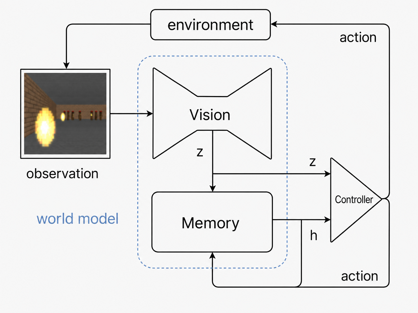
Vision Model: Compressing What We See

At each time step, the agent receives a high-dimensional observation \(x_t\), for example, high-resolution images. The task of Vision Model (V) is to compress this observation into a low-dimensional latent representation:

In the original paper, V is implemented as a variational autoencoder. The encoder maps an image into a latent vector \(z_t\), while the decoder tries to reconstruct the original image from it.

This compression is deliberately lossy. The reconstructed image does not preserve every pixel of the original frame, nor does it need to. What matters is that \(z_t\) keeps enough information to represent the visually important structure of the current observation.

In this sense, operating on this kind of internally constructed representation instead of the raw observation itself may answer the question we raised earlier. However, there is still an obvious problem. Suppose we show the agent a single image of a car on a racing track. From \(z_t\), it may know roughly where the car and the road are. But a single image does not tell us whether the car is moving quickly or slowly, whether it is turning left or right, or how its current motion will affect what happens next. In other words, \(z_t\) compresses what is currently seen, but a world is not just a collection of static scenes. Therefore, in addition to compressing space, the agent also needs to compress time. Since the system evolves over time, one way to achieve this is to record the evolving history, i.e., memory.

Memory Model: Compressing What Happens over Time

At every time step, the Memory Model (M) receives the current latent observation \(z_t\), the action \(a_t\) taken by the agent, and its current internal memory \(h_t\). This module has two output heads, one for updating memory:

where \(h_t\) can be roughly understood as a compressed summary of information accumulated from the past; the other for predicting the possible next state in the latent space. Within the internal memory as extra input, the world model learns to output a probability distribution:

This gives us a much more interesting notion of a state. We may therefore roughly regard

as the agent’s internal description of its present situation. One part tells it what the world looks like now. The other tells it how the world has been evolving, which contains predictive temporal information unavailable from a single observation.

There is a subtle point here that I find especially interesting. The agent does not always need to explicitly generate several possible futures, inspect them one by one, and then choose the best action. If the predictive structure of the future has already been compressed into \(h_t\), the controller may simply learn to react to that representation. In other words, prediction can affect action even without explicit rollout.

Recall the distinction between planning and reacting we discussed in the previous section. A skilled driver does not consciously simulate every possible trajectory before turning the steering wheel. Years of experience allow information about future consequences to be embedded in the driver’s current perception and reflexes. The paper suggests a computational analogue of this idea: a predictive model of the future can provide useful features for a reactive policy, even when the policy does not explicitly “think several steps ahead”.

Controller: Acting through the Internal World

Compared with V and M, the Controller (C) is surprisingly simple. In the original paper, it’s only a linear mapping from the current latent representation and the memory state to an action:

Most of the complexity of the agent resides in the world model rather than in the policy itself. V learns how observations should be represented; M learns how this representation evolves over time; C only needs to learn how to act based on the representations already produced by V and M. Putting these three components together, interaction with the environment looks roughly like

The real environment then executes \(a_t\) and returns the next observation \(x_{t+1}\), and this loop continues.

At first glance, this may look like little more than an unusual architecture for reinforcement learning. But the predictive distribution produced by M introduces a much more radical possibility. If M can tell us what the next latent state is likely to be, why must we ask the real environment for \(x_{t+1}\) at all?

Learning Inside the Dream

Suppose at time \(t\), instead of performing \(a_t\) in the real world, we ask M to predict what would happen:

Now treat this sampled \(z_{t+1}\) as if it were the next observation. Then the controller chooses another action \(a_{t+1}\), M predicts another latent state:

We can continue to rollout in this manner, thus resulting in a trajectory:

We call this kind of latent imagination, a dream. If an agent can act inside such a dream, can it also learn inside it?

The VizDoom experiment pushes the idea much further. The task is simple: the agent needs to avoid fireballs and survive for as long as possible. To turn M into something that can replace the original game environment, the authors extend it slightly. Besides predicting the next latent observation, M also predicts whether the agent will die:

where \(d_{t+1}\) indicates whether the episode terminates. With this addition, the learned model contains enough information to expose an interface similar to the original reinforcement-learning environment. The controller can choose an action, receive a new latent state, and eventually receive a termination signal—all without running the actual game engine.

The training procedure can therefore be separated into two stages:

1. Collect experience from the real world and learn the model;
2. Remove the real world and train the controller inside the learned one;
3. Finally, put the controller back into the actual environment.

And remarkably, this works. The controller trained entirely in the generated VizDoom environment transfers back to the real game and successfully solves the task.

Recall that Dyna used the model to generate \(k\) hypothetical experiences in addition to every real experience. This experiment pushes \(k\) toward an extreme. Once enough real data has been used to learn the model, the agent can stop interacting with reality altogether and perform its subsequent policy learning inside the model. So the world model is no longer merely an auxiliary component that provides additional samples. It becomes an alternative environment in which learning itself can take place.

Perhaps machines do not need to imagine in the raw sensory world at all. They can learn a compressed latent space, learn its dynamics, and then perform their imagination directly inside that space. The world that matters to the agent does not have to be the world as rendered in pixels. It can be an internal world expressed in a language convenient for prediction and control.

Hazy Dreams

Remember that the vision model is implemented as a VAE, which learns its representation largely by reconstructing observations. This provides a useful and general latent space, but reconstruction itself does not tell us which aspects of the world actually matter for intelligent behavior. For example, a texture on the wall may require many bits to reconstruct accurately but be irrelevant to the task; the position of a small obstacle may occupy only a few pixels but completely determine whether the next action succeeds or fails.

So we arrive at some deeper questions: What should that latent world contain in the first place? Should a world model try to preserve and predict everything it observes? Or should it deliberately ignore some parts of reality and retain only the structures useful for understanding, prediction, and action?

What should machines imagine?

Since we’ve already discussed that learning the world model is a spatial-temporal task, a video prediction scenario would be perfect for explaining the formalized idea. Suppose the system is given two video clips in order, and the goal is to tell what degree the second video clip (denoted as \(y\)) is a plausible continuation of the first one (denoted as \(x\)). The reason we didn’t impose the model to predict \(y\) directly from \(x\) is because there is an infinite number of plausible continuations of a given clip. But it’s tractable for the system to evaluate if a proposed \(y\) is compatible with a given \(x\). And a general framework of the model to achieve this is the Energy-Based Models (EBMs).

Energy-Based Models with Latent Variables

Intuitively, we can formally learn a scalar-valued function \(F(x,y)\) that produces low energy values when \(x\) and \(y\) are compatible and higher values when they are not. That seems promising, but the difficulty lies in the fact that the future is not fully predictable from the past. Consider a car approaching a fork in the road. From the current observation, the car may plausibly turn left or turn right; choosing either option is reasonable.

It is evident that some information influencing the future is not contained in \(x\); therefore, we use a latent variable, denoted as \(z\), to represent this missing information. Thus the predictor can be formed as:

where \(\theta\) is the parameter vector of the neural network that computes the energy function \(F_w(x,y)\), defined as:

where \(E\) is some qualified energy function. When the future \(y\) is known, for example during training, we can find an exist \(z\) such that the model explains \(y\) well based on \(x\). When the future \(y\) has not yet been observed, we can enumerate different values ​​of \(z\in\mathcal{Z}\) or sample \(z\) from a probability distribution to generate multiple candidate futures.

So how do we train this EBM?

Given a dataset:

where each pair \((x_i,y_i)\) is an observed compatible combination. We hope to learn an parameterized energy function \(F_\theta(x,y)\) that satisfies the property mentioned earlier.

To achieve that, we need to devise a loss function \(\mathcal{L}\), such that given a training sample \((x,y)\), minimizing this loss will make the energy \(F_\theta(x,y)\) lower than the energies \(F_\theta(x,y^\prime)\) of any \(y^\prime\) different from \(y\). Note that the energy function and the training loss are distinct entities. The energy function evaluates a candidate, whereas the training loss assesses whether that energy function distinguishes sufficiently well between different types of candidates. There’re usually two kinds of methods to design the loss function. One is called contrastive methods, and the other is called regularized methods.

JEPA

Even if we somehow knew that the car would turn left, there would still be countless details that are difficult or impossible to predict exactly: the movement of leaves, subtle lighting changes, the precise texture appearing on the road, or the exact configuration of distant objects. However, this is the wrong burden to place on a world model. A world model intended for intelligent behavior may not need to know what every leaf will look like one second later. It may only need to know that there is a tree over there, while allocating much more capacity to something like the vehicle ahead may enter my lane.

In other words, part of intelligence may consist not only in predicting the future, but also in learning which parts of the future are worth predicting. This suggests a different objective. Instead of predicting \(y\), perhaps the system should predict an abstract representation of \(y\), denoted as \(s_y\), in which important aspects of the world remain, while irrelevant and unpredictable details disappear?

This is the basic motivation behind Joint Embedding Predictive Architecture (JEPA).

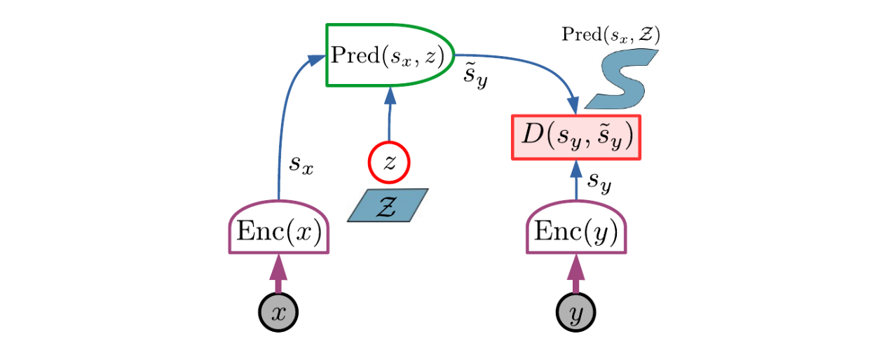
A generic JEPA contains three important pieces.

1. Firstly, the two variables \(x\) and \(y\) are fed to two distinct encoders, producing two latent presentations \(s_x\) and \(s_y\). Since the two encoders are not necessarily identical, \(x\) and \(y\) may represent different types of information (e.g. video and audio);
2. Then a predictor tries to predict the representation of \(y\) from the representation of \(x\) and optionaly a latent variable \(z\);
3. Finally, the prediction is evaluated by comparing representations: \(E_\theta(x,y,z)=D\left(s_y,\operatorname{Pred}(s_x,z)\right)\), where \(D\) measures the discrepancy between the actual representation and its predicted representation.

Since JEPA performs predictions in reperesentation space, the two encoders are free to discard information that is not useful for prediction, e.g. irrelevant details.

The Training of JEPA

As we’ve talked about, we use two separate encoders to get latent representations \(s_x\) and \(s_y\), which offers great flexibility, but also gives rise to the collapse problem.

References

[1] Richard S. Sutton. Integrated Architectures for Learning, Planning, and Reacting Based on Approximating Dynamic Programming. Machine Learning Proceedings 1990, 216-224 (1990).

[2] Ha, David and Schmidhuber, Jürgen. World Models. Zenodo (2018). https://doi.org/10.5281/zenodo.1207631

[3] Yann LeCun and Courant. A Path Towards Autonomous Machine Intelligence. (2022).